Article Source
- Title: Deep Learning
- Source: Wikipedia, the free encyclopedia
Deep learning
Deep learning is a set of algorithms in machine learning that attempt to model high-level abstractions in data by using architectures composed of multiple non-linear transformations.[1]
Deep learning is part of a broader family of machine learning methods based on learning representations. An observation (e.g., an image) can be represented in many ways (e.g., a vector of pixels), but some representations make it easier to learn tasks of interest (e.g., is this the image of a human face?) from examples, and research in this area attempts to define what makes better representations and how to create models to learn these representations.
Various deep learning architectures such as deep neural networks, convolutional deep neural networks, and deep belief networks have been applied to fields like computer vision, automatic speech recognition, natural language processing, and music/audio signal recognition where they have been shown to produce state-of-the-art results on various tasks.
Contents
- 1 Introduction
- 2 Fundamental concepts
- 3 Deep learning in artificial neural networks
- 4 Deep learning architectures
- 5 Deep learning in the human brain
- 6 Publicity around deep learning
- 7 Criticisms
- 8 See also
- 9 References
- 10 External links
Introduction
Deep learning architectures, specifically those built from artificial neural networks (ANN), date back at least to the Neocognitron introduced by Kunihiko Fukushima in 1980.[2] The ANNs themselves date back even further. In 1989, Yann LeCun et al. were able to apply the standard backpropagation algorithm, which had been around since 1974,[3] to a deep neural network with the purpose of recognizing handwritten zip codes on mail. Despite the success of applying the algorithm, the time to train the network on this dataset was approximately 3 days, making it impractical for general use.[4] Many factors contribute to the slow speed, one being due to the so-called vanishing gradient problem analyzed in 1991 by Jürgen Schmidhuber’s student Sepp Hochreiter.[5][6] In combination with speed issues, ANNs fell out of favor in practical machine learning and simpler models such as support vector machines (SVMs) became the popular choice of the field in the 1990s and 2000s.
The term “deep learning” gained traction in the mid-2000s after a publication by Geoffrey Hinton and Ruslan Salakhutdinov showed how a many-layered feedforward neural network could be effectively pre-trained one layer at a time, treating each layer in turn as an unsupervised restricted Boltzmann machine, then using supervised backpropagation for fine-tuning.[7] In 1992, Schmidhuber had already implemented a very similar idea for the more general case of unsupervised deep hierarchies of recurrent neural networks, and also experimentally shown its benefits for speeding up supervised learning [8][9]
Since the resurgence of deep learning, it has shown to be part of many state-of-the-art systems in different disciplines, particularly that of computer vision and automatic speech recognition (ASR). Results on commonly used evaluation sets such as TIMIT (ASR) and MNIST (image classification) are constantly being improved with new applications of deep learning. Currently, it has been shown that deep learning architectures in the form of convolution neural networks have been best performing, however, these are more widely used in computer vision than in ASR.
Advances in hardware have also been an important enabling factor for the renewed interest of deep learning. In particular, powerful graphics processing units (GPUs) are highly suited for the kind of number crunching, matrix/vector math involved in machine learning. GPUs have been shown to speed up training algorithms by orders of magnitude, bringing running times of weeks back to days.[10][11]
Fundamental concepts
Deep learning algorithms are based on distributed representations, a concept used in machine learning. The underlying assumption behind distributed representations is that observed data is generated by the interactions of many different factors on different levels. Deep learning adds the assumption that these factors are organized into multiple levels, corresponding to different levels of abstraction or composition. Varying numbers of layers and layer sizes can be used to provide different amounts of abstraction.[1]
Deep learning algorithms in particular exploit this idea of hierarchical explanatory factors. Different concepts are learned from other concepts, with the more abstract, higher level concepts being learned from the lower level ones. These architectures are often constructed with a greedy layer-by-layer method that models this idea. Deep learning helps to disentangle these abstractions and pick out which features are useful for learning.[1]
Many deep learning algorithms are actually framed as unsupervised learning problems. Because of this, these algorithms can make use of the unlabeled data that other algorithms cannot. Unlabeled data is usually more abundant than labeled data, making this a very important benefit of these algorithms. The deep belief network introduced in the next section is an example of a deep structure that can be trained in an unsupervised manner.[1]
Deep learning in artificial neural networks
Some of the most successful deep learning methods involve artificial neural networks. Artificial neural networks are inspired by the 1959 biological model proposed by Nobel laureates David H. Hubel & Torsten Wiesel, who found two types of cells in the visual primary cortex: simple cells and complex cells. Many artificial neural networks can be viewed as cascading models[12] of cell types inspired by these biological observations.
Fukushima’s Neocognitron introduced convolutional neural networks partially trained by unsupervised learning. Yann LeCun et al. (1989) applied supervised backpropagation to such architectures.[13]
With the advent of the back-propagation algorithm in the 1970s, many researchers tried to train supervised deep artificial neural networks from scratch, initially with little success. Sepp Hochreiter’s diploma thesis of 1991[14][15] formally identified the reason for this failure in the “vanishing gradient problem,” which not only affects many-layered feedforward networks, but also recurrent neural networks. The latter are trained by unfolding them into very deep feedforward networks, where a new layer is created for each time step of an input sequence processed by the network. As errors propagate from layer to layer, they shrink exponentially with the number of layers.
To overcome this problem, several methods were proposed. One is Jürgen Schmidhuber’s multi-level hierarchy of networks (1992) pre-trained one level at a time through unsupervised learning, fine-tuned through backpropagation.[8] Here each level learns a compressed representation of the observations that is fed to the next level.
Another method is the long short term memory (LSTM) network of 1997 by Hochreiter & Schmidhuber.[16] In 2009, deep multidimensional LSTM networks demonstrated the power of deep learning with many nonlinear layers, by winning three ICDAR 2009 competitions in connected handwriting recognition, without any prior knowledge about the three different languages to be learned.[17][18]
Sven Behnke relied only on the sign of the gradient (Rprop) when training his Neural Abstraction Pyramid[19] to solve problems like image reconstruction and face localization.
Other methods also use unsupervised pre-training to structure a neural network, making it first learn generally useful feature detectors. Then the network is trained further by supervised back-propagation to classify labeled data. The deep model of Hinton et al. (2006) involves learning the distribution of a high level representation using successive layers of binary or real-valued latent variables. It uses a restricted Boltzmann machine (Smolensky, 1986[20]) to model each new layer of higher level features. Each new layer guarantees an increase on the lower-bound of the log likelihood of the data, thus improving the model, if trained properly. Once sufficiently many layers have been learned the deep architecture may be used as a generative model by reproducing the data when sampling down the model (an “ancestral pass”) from the top level feature activations.[21] Hinton reports that his models are effective feature extractors over high-dimensional, structured data.[22]
The Google Brain team led by Andrew Ng and Jeff Dean created a neural network that learned to recognize higher-level concepts, such as cats, only from watching unlabeled images taken from YouTube videos.[23] [24]
Other methods rely on the sheer processing power of modern computers, in particular, GPUs. In 2010 it was shown by Dan Ciresan and colleagues[10] in Jürgen Schmidhuber’s group at the Swiss AI Lab IDSIA that despite the above-mentioned “vanishing gradient problem,” the superior processing power of GPUs makes plain back-propagation feasible for deep feedforward neural networks with many layers. The method outperformed all other machine learning techniques on the old, famous MNIST handwritten digits problem of Yann LeCun and colleagues at NYU.
As of 2011, the state of the art in deep learning feedforward networks alternates convolutional layers and max-pooling layers,[25][26] topped by several pure classification layers. Training is usually done without any unsupervised pre-training. Since 2011, GPU-based implementations[25] of this approach won many pattern recognition contests, including the IJCNN 2011 Traffic Sign Recognition Competition,[27] the ISBI 2012 Segmentation of neuronal structures in EM stacks challenge,[28] and others.
Such supervised deep learning methods also were the first artificial pattern recognizers to achieve human-competitive performance on certain tasks.[29]
Deep learning architectures
It is worth explaining some common architectures used for deep learning. Basic models of deep neural networks and deep belief networks are given below.
Deep neural networks
A deep neural network (DNN) is defined to be an artificial neural network with at least one hidden layer of units between the input and output layers, it is also a universal approximator.[30] Similar to shallow ANNs, it can model complex non-linear relationships. The extra layers give it added levels of abstraction, thus increasing its modeling capability. DNNs are typically designed as feedforward networks, but recent research has successfully applied the deep learning architecture to recurrent neural networks for applications such as language modeling.[31] Convolutional deep neural networks (CNNs) are used in computer vision where their success is well-documented.[32] More recently, CNNs have been applied to acoustic modeling for automatic speech recognition (ASR), where they have shown success over previous models.[33] For simplicity, a look at training DNNs is given here.
A DNN can be discriminatively trained with the standard backpropagation algorithm. The weight updates can be done via stochastic gradient descent using the following equation:

Here,  is the learning rate, and
  is the cost function. The choice
of the cost function depends on factors such as the learning type
(supervised, unsupervised, reinforcement, etc.) and the activation
function. For example,
when performing supervised learning on a multiclass classification
problem, common choices for the activation function and cost function
are the
softmax
function and cross entropy
function, respectively. The softmax function is defined as
is the cost function. The choice
of the cost function depends on factors such as the learning type
(supervised, unsupervised, reinforcement, etc.) and the activation
function. For example,
when performing supervised learning on a multiclass classification
problem, common choices for the activation function and cost function
are the
softmax
function and cross entropy
function, respectively. The softmax function is defined as 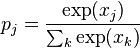 where
where  represents the class probability and
  and
and  represent the total input to units
  and
and  respectively. Cross-entropy is defined as
 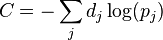 where
where  represents the target probability for output unit
and
is the probability output for
after applying the activation
function.[34]
represents the target probability for output unit
and
is the probability output for
after applying the activation
function.[34]
Issues with deep neural networks
Like with ANNs, many issues can arise with DNNs if they are naively trained. Two common issues are overfitting and computation time.
DNNs are very prone to overfitting because of the added layers of
abstraction, which allow them to model rare dependencies in the training
data. Regularization methods
such as weight decay ( -regularization)
or sparsity (
-regularization)
or sparsity ( -regularization)
can be applied during training to help combat
overfitting.[35] Another regularization
method that has been more recently applied to DNNs is “dropout”
regularization. In dropout, some number of units are randomly omitted
from the hidden layers during training. This helps to break the rare
dependencies that can occur in the training data
[36]
-regularization)
can be applied during training to help combat
overfitting.[35] Another regularization
method that has been more recently applied to DNNs is “dropout”
regularization. In dropout, some number of units are randomly omitted
from the hidden layers during training. This helps to break the rare
dependencies that can occur in the training data
[36]
Backpropagation and gradient descent have been the preferred method for training these structures due to the ease of implementation and their tendency to converge to better local optima in comparison with other training methods. However, these methods can be very computationally expensive, especially when being used to train DNNs. There are many parameters to be considered with a DNN, such as the size (number of layers and number of units per layer), the learning rate, initial weights, etc. Sweeping through the parameters may not be feasible in many tasks due to the time cost. Various ‘tricks’ such as using mini-batching (computing the gradient on several training examples at once rather than individual examples) [37] have been shown to speed up computation. The sheer processing power of GPUs arguably has shown the most significant speed up, mainly due to the matrix and vector computations required being well suited for GPUs. However, it is hard to make use of large cluster machines for training DNNs, so better methods of parallelizing training will undoubtedly give a significant speed up as well.
Deep belief networks
Main article: Deep belief network

An restricted Boltzmann machine (RBM _with fully connected visible and hidden units. Note there are no hidden-hidden or visible-visible connections.
A deep belief network (DBN) is a probabilistic, generative model made up of multiple layers of hidden units. It can be looked at as a composition of simple learning modules that make up each layer.[38]
A DBN can be used for generatively pre-training a DNN by using the learned weights as the initial weights. Backpropagation or other discriminative algorithms can then be applied for fine-tuning of these weights. This is particularly helpful in situations where limited training data is available, as poorly initialized weights can have significant impact on the performance of the final model. These pre-trained weights are in a region of the weight space that is closer to the optimal weights (as compared to just random initialization). This allows for both improved modeling capability and faster convergence of the fine-tuning phase.[39]
A DBN can be efficiently trained in an unsupervised, layer-by-layer manner where the layers are typically made of restricted Boltzmann machines (RBM). A description of training a DBN via RBMs is provided below. An RBM is an undirected, generative energy-based model with an input layer and single hidden layer. Connections only exist between the visible units of the input layer and the hidden units of the hidden layer; there are no visible-visible or hidden-hidden connections.
The training method for RBMs was initially proposed by Geoffrey Hinton for use with training “Product of Expert” models and is known as contrastive divergence (CD).[40] CD provides an approximation to the maximum likelihood method that would ideally be applied for learning the weights of the RBM.[37]
In training a single RBM, weight updates are performed with gradient
ascent via the following
equation:  .
Here,
.
Here,
 is the probability of a visible vector, which is given by
  .
.
 is the partition function (used for normalizing) and
 is the energy function assigned to the state of the network. A lower
energy indicates the network is in a more “desirable” configuration. The
gradient
is the energy function assigned to the state of the network. A lower
energy indicates the network is in a more “desirable” configuration. The
gradient  has the simple form
  where
where
 represent averages with respect to distribution
 .
The issue arises in sampling
.
The issue arises in sampling  as this requires running alternating Gibbs
sampling for a long time. CD
replaces this step by running alternating Gibbs sampling for
as this requires running alternating Gibbs
sampling for a long time. CD
replaces this step by running alternating Gibbs sampling for
 steps (values of
  have empirically been shown to perform well). After
steps, the data is sampled and that sample is used in place of
.
The CD procedure works as follows:[37]
have empirically been shown to perform well). After
steps, the data is sampled and that sample is used in place of
.
The CD procedure works as follows:[37]
- Initialize the visible units to a training vector.
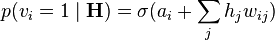
- Update the hidden units in parallel given the visible units:
 .
.
 represents the sigmoid function and
 is the bias of
 .
. - Update the visible units in parallel given the hidden units:
 .
.
 is the bias of
 .
This is called the “reconstruction” step.
.
This is called the “reconstruction” step. - Reupdate the hidden units in parallel given the reconstructed visible units using the same equation as in step 2.
- Perform the weight update:
 .
.
Once an RBM is trained, another RBM can be “stacked” atop of it to create a multilayer model. Each time another RBM is stacked, the input visible layer is initialized to a training vector and values for the units in the already-trained RBM layers are assigned using the current weights and biases. The final layer of the already-trained layers is used as input to the new RBM. The new RBM is then trained with the procedure above, and then this whole process can be repeated until some desired stopping criterion is met.[41]
Despite the approximation of CD to maximum likelihood being very crude (CD has been shown to not follow the gradient of any function), empirical results have shown it to be an effective method for use with training deep architectures.[37]
Convolutional neural networks
Main article: Convolutional neural network
A CNN is composed of one or more convolutional layers with fully connected layers (matching those in typical artificial neural networks) on top. It also uses tied weights and pooling layers. This architecture allows CNNs to take advantage of the 2D structure of input data. In comparison with other deep architectures, convolutional neural networks are starting to show superior results in both image and speech applications. They can also be trained with standard backpropagation. CNNs are easier to train than other regular, deep, feed-forward neural networks and have many fewer parameters to estimate, making them a highly attractive architecture to use.[42]
Convolutional Deep Belief Networks
Arguably the most recent achievement in deep learning is from the use of convolutional deep belief networks (CDBN). A CDBN is very similar to normal Convolutional neural network in terms of its structure. Therefore, like CNNs they are also able to exploit the 2D structure of images combined with the advantage gained by pre-training in Deep belief network. They provide a generic structure which can be used in many image and signal processing tasks and can be trained in a way similar to that for Deep Belief Networks. Recently, many benchmark results on standard image datasets like CIFAR [43] have been obtained using CDBNs.[44]
Results
Automatic speech recognition
The results shown in the table below are for automatic speech recognition on the popular TIMIT data set. This is a common data set used for initial evaluations of deep learning architectures. The entire set contains 630 speakers from eight major dialects of American English, with each speaker reading 10 different sentences.[45] Its small size allows many different configurations to be tried effectively with it. The error rates presented are phone error rates (PER).
| Method | PER (%) |
|---|---|
| Randomly Initialized RNN | 26.1 |
| Bayesian Triphone GMM-HMM | 25.6 |
| Monophone Randomly Initialized DNN | 23.4 |
| Monophone DBN-DNN | 22.4 |
| Triphone GMM-HMM with BMMI Training | 21.7 |
| Monophone DBN-DNN on fbank | 20.7 |
| Convolutional DNN | 20.0 |
Image classification
A common evaluation set for image classification is the MNIST database data set. MNIST is composed of handwritten digits and includes 60000 training examples and 10000 test examples. Similar to TIMIT, its small size allows multiple configurations to be tested. A comprehensive list of results on this set can be found in.[46] The current best result on MNIST is an error rate of 0.23%, achieved by Ciresan et al. in 2012.[47]
Deep learning in the human brain
Computational deep learning is closely related to a class of theories of brain development (specifically, neocortical development) proposed by cognitive neuroscientists in the early 1990s.[48] The most approachable summary of this work is Elman, et al.’s 1996 book “Rethinking Innateness” [49] (see also: Shrager and Johnson;[50] Quartz and Sejnowski [51]). As these theories were also instantiated in computational models, they are technical predecessors of purely computationally-motivated deep learning models. These models share the interesting property that various proposed learning dynamics in the brain (e.g., a wave of neurotrophic growth factor) conspire to support the self-organization of just the sort of inter-related neural networks utilized in the later, purely computational deep learning models, and which appear to be analogous to one way of understanding the neocortex of the brain as a hierarchy of filters where each layer captures some of the information in the operating environment, and then passes the remainder, as well as modified base signal, to other layers further up the hierarchy. The result of this process is a self-organizing stack of transducers, well-tuned to their operating environment. As described in The New York Times in 1995: “…the infant’s brain seems to organize itself under the influence of waves of so-called trophic-factors … different regions of the brain become connected sequentially, with one layer of tissue maturing before another and so on until the whole brain is mature.” [52]
The importance of deep learning with respect to the evolution and development of human cognition did not escape the attention of these researchers. One aspect of human development that distinguishes us from our nearest primate neighbors may be changes in the timing of development.[53] Among primates, the human brain remains relatively plastic until late in the post-natal period, whereas the brains of our closest relatives are more completely formed by birth. Thus, humans have greater access to the complex experiences afforded by being out in the world during the most formative period of brain development. This may enable us to “tune in” to rapidly changing features of the environment that other animals, more constrained by evolutionary structuring of their brains, are unable to take account of. To the extent that these changes are reflected in similar timing changes in hypothesized wave of cortical development, they may also lead to changes in the extraction of information from the stimulus environment during the early self-organization of the brain. Of course, along with this flexibility comes an extended period of immaturity, during which we are dependent upon our caretakers and our community for both support and training. The theory of deep learning therefore sees the coevolution of culture and cognition as a fundamental condition of human evolution.[54]
Publicity around deep learning
Deep learning is often presented as a step towards realising strong AI[55] and thus many organizations have become interested in its use for particular applications. Most recently, in December 2013, Facebook announced that it hired Yann LeCun to head its new artificial intelligence (AI) lab that will have operations in California, London, and New York. The AI lab will be used for developing deep learning techniques that will help Facebook do tasks such as automatically tagging uploaded pictures with the names of the people in them.[56]
In March 2013, Geoffrey Hinton and two of his graduate students, Alex Krizhevsky and Ilya Sutskever, were hired by Google. Their work will be focused on both improving existing machine learning products at Google and also help deal with the growing amount of data Google has. Google also purchased Hinton’s company, DNNresearch, for an undisclosed sum of money.
Criticisms
A main criticism of deep learning concerns the lack of theory surrounding many of the methods. Most of the learning in deep architectures is just some form of gradient descent. While gradient descent has been understood for a while now, the theory surrounding other algorithms, such as contrastive divergence is less clear (i.e., Does it converge? If so, how fast? What is it approximating?). Deep learning methods are often looked at as a black box, with most confirmations done empirically, rather than theoretically.
Others point out that deep learning should be looked at as a step towards realizing strong AI, not as an all-encompassing solution. Despite the power of deep learning methods, they still lack much of the functionality needed for realizing this goal entirely. Research psychologist Gary Marcus has noted that:
“Realistically, deep learning is only part of the larger challenge of building intelligent machines. Such techniques lack ways of representing causal relationships (…) have no obvious ways of performing logical inferences, and they are also still a long way from integrating abstract knowledge, such as information about what objects are, what they are for, and how they are typically used. The most powerful A.I. systems, like Watson (…) use techniques like deep learning as just one element in a very complicated ensemble of techniques, ranging from the statistical technique of Bayesian inference to deductive reasoning.” [57]
See also
- Graphical model
- Applications of artificial intelligence
- Andrew Ng
- List of artificial intelligence projects
- Center for Biological and Computational Learning at MIT
References
- \ a b c d Y. Bengio, A. Courville, and P. Vincent., “Representation Learning: A Review and New Perspectives,” IEEE Trans. PAMI, special issue Learning Deep Architectures, 2013
- [](#cite_ref-FUKU1980_2-0) K. Fukushima., “Neocognitron: A self-organizing neural network model for a mechanism of pattern recognition unaffected by shift in position,” Biol. Cybern., 36, 193–202, 1980
- [](#cite_ref-WERBOS1974_3-0) P. Werbos., “Beyond Regression: New Tools for Prediction and Analysis in the Behavioral Sciences,” PhD thesis, Harvard University, 1974.
- [](#cite_ref-LECUN1989_4-0) LeCun et al., “Backpropagation Applied to Handwritten Zip Code Recognition,” Neural Computation, 1, pp. 541–551, 1989.
- [](#cite_ref-HOCH1991_5-0) S. Hochreiter., “Untersuchungen zu dynamischen neuronalen Netzen,” Diploma thesis. Institut f. Informatik, Technische Univ. Munich. Advisor: J. Schmidhuber, 1991.
- [](#cite_ref-HOCH2001_6-0) S. Hochreiter et al., “Gradient flow in recurrent nets: the difficulty of learning long-term dependencies,” In S. C. Kremer and J. F. Kolen, editors, A Field Guide to Dynamical Recurrent Neural Networks. IEEE Press, 2001.
- [](#cite_ref-HINTON2007_7-0) G. E. Hinton., “Learning multiple layers of representation,” Trends in Cognitive Sciences, 11, pp. 428–434, 2007.
- \ a b J. Schmidhuber., “Learning complex, extended sequences using the principle of history compression,” Neural Computation, 4, pp. 234–242, 1992.
- [](#cite_ref-SCHMID1991_9-0) J. Schmidhuber., “My First Deep Learning System of 1991 + Deep Learning Timeline 1962–2013.”
- \ a b D. C. Ciresan et al., “Deep Big Simple Neural Nets for Handwritten Digit Recognition,” Neural Computation, 22, pp. 3207–3220, 2010.
- [](#cite_ref-RAINA2009_11-0) R. Raina, A. Madhavan, A. Ng., “Large-scale Deep Unsupervised Learning using Graphics Processors,” Proc. 26th Int. Conf. on Machine Learning, 2009.
- [](#cite_ref-12) M Riesenhuber, T Poggio. Hierarchical models of object recognition in cortex. Nature neuroscience, 1999(11) 1019–1025.
- [](#cite_ref-LeCun1989_13-0) Y. LeCun, B. Boser, J. S. Denker, D. Henderson, R. E. Howard, W. Hubbard, L. D. Jackel. Backpropagation Applied to Handwritten Zip Code Recognition. Neural Computation, 1(4):541–551, 1989.
- [](#cite_ref-14) S. Hochreiter. Untersuchungen zu dynamischen neuronalen Netzen. Diploma thesis, Institut f. Informatik, Technische Univ. Munich, 1991. Advisor: J. Schmidhuber
- [](#cite_ref-15) S. Hochreiter, Y. Bengio, P. Frasconi, and J. Schmidhuber. Gradient flow in recurrent nets: the difficulty of learning long-term dependencies. In S. C. Kremer and J. F. Kolen, editors, A Field Guide to Dynamical Recurrent Neural Networks. IEEE Press, 2001.
- [](#cite_ref-lstm_16-0) Hochreiter, Sepp; and Schmidhuber, Jürgen; Long Short-Term Memory, Neural Computation, 9(8):1735–1780, 1997
- [](#cite_ref-17) Graves, Alex; and Schmidhuber, Jürgen; Offline Handwriting Recognition with Multidimensional Recurrent Neural Networks, in Bengio, Yoshua; Schuurmans, Dale; Lafferty, John; Williams, Chris K. I.; and Culotta, Aron (eds.), Advances in Neural Information Processing Systems 22 (NIPS’22), December 7th–10th, 2009, Vancouver, BC, Neural Information Processing Systems (NIPS) Foundation, 2009, pp. 545–552
- [](#cite_ref-18) A. Graves, M. Liwicki, S. Fernandez, R. Bertolami, H. Bunke, J. Schmidhuber. A Novel Connectionist System for Improved Unconstrained Handwriting Recognition. IEEE Transactions on Pattern Analysis and Machine Intelligence, vol. 31, no. 5, 2009.
- [](#cite_ref-19) Sven Behnke (2003). Hierarchical Neural Networks for Image Interpretation.. Lecture Notes in Computer Science 2766. Springer.
- [](#cite_ref-smolensky1986_20-0) Smolensky, P. (1986). “Information processing in dynamical systems: Foundations of harmony theory.”. In D. E. Rumelhart, J. L. McClelland, & the PDP Research Group, Parallel Distributed Processing: Explorations in the Microstructure of Cognition. 1. pp. 194–281.
- [](#cite_ref-hinton2006_21-0) Hinton, G. E.; Osindero, S.; Teh, Y. (2006). “A fast learning algorithm for deep belief nets”. Neural Computation 18 (7): 1527–1554. doi:10.1162/neco.2006.18.7.1527. PMID 16764513.
- [](#cite_ref-22) Hinton, G. (2009). “Deep belief networks”. Scholarpedia 4 (5): 5947. doi:10.4249/scholarpedia.5947. edit
- [](#cite_ref-markoff2012_23-0) John Markoff (25 June 2012). “How Many Computers to Identify a Cat? 16,000.”. New York Times.
- [](#cite_ref-ng2012_24-0) Ng, Andrew; Dean, Jeff (2012). “Building High-level Features Using Large Scale Unsupervised Learning”.
- \ a b D. C. Ciresan, U. Meier, J. Masci, L. M. Gambardella, J. Schmidhuber. Flexible, High Performance Convolutional Neural Networks for Image Classification. International Joint Conference on Artificial Intelligence (IJCAI-2011, Barcelona), 2011.
- [](#cite_ref-martines2013_26-0) Martines, H., Bengio, Y., & Yannakakis, G. N. (2013). Learning Deep Physiological Models of Affect. I EEE Computational Intelligence, 8(2), 20.
- [](#cite_ref-ciresan2011NN_27-0) D. C. Ciresan, U. Meier, J. Masci, J. Schmidhuber. Multi-Column Deep Neural Network for Traffic Sign Classification. Neural Networks, 2012.
- [](#cite_ref-ciresan2012NIPS_28-0) D. Ciresan, A. Giusti, L. Gambardella, J. Schmidhuber. Deep Neural Networks Segment Neuronal Membranes in Electron Microscopy Images. In Advances in Neural Information Processing Systems (NIPS 2012), Lake Tahoe, 2012.
- [](#cite_ref-ciresan2011CVPR_29-0) D. C. Ciresan, U. Meier, J. Schmidhuber. Multi-column Deep Neural Networks for Image Classification. IEEE Conf. on Computer Vision and Pattern Recognition CVPR 2012.
- [](#cite_ref-30) http://deeplearning.net/tutorial/mlp.html
- [](#cite_ref-MIKO2010_31-0) T. Mikolov et al., “Recurrent neural network based language model,” Interspeech, 2010.
- [](#cite_ref-LECUN86_32-0) Y. LeCun et al., “Gradient-based learning applied to document recognition,” Proceedings of the IEEE, 86 (11), pp. 2278–2324.
- [](#cite_ref-SAIN2013_33-0) T. Sainath et al., “Convolutional neural networks for LVCSR,” ICASSP, 2013.
- [](#cite_ref-HINTON2012_34-0) G. E. Hinton et al., “Deep Neural Networks for Acoustic Modeling in Speech Recognition: The shared views of four research groups,” IEEE Signal Processing Magazine, pp. 82–97, November 2012.
- [](#cite_ref-BENGIO2013_35-0) Y. Bengio et al., “Advances in optimizing recurrent networks,” ICASSP’, 2013.
- [](#cite_ref-DAHL2013_36-0) G. Dahl et al., “Improving DNNs for LVCSR using rectified linear units and dropout,” ICASSP’, 2013.
- \ a b c d G. E. Hinton., “A Practical Guide to Training Restricted Boltzmann Machines,” Tech. Rep. UTML TR 2010-003, Dept. CS., Univ. of Toronto, 2010.
- [](#cite_ref-SCHOLARDBNS_38-0) G.E. Hinton., “Deep belief networks,” Scholarpedia, 4(5):5947.
- [](#cite_ref-LAROCH2007_39-0) H. Larochelle et al., “An empirical evaluation of deep architectures on problems with many factors of variation,” in Proc. 24th Int. Conf. Machine Learning, pp. 473–480, 2007.
- [](#cite_ref-POE_40-0) G. E. Hinton., “Training Product of Experts by Minimizing Contrastive Divergence,” Neural Computation, 14, pp. 1771–1800, 2002.
- [](#cite_ref-BENGIODEEP_41-0) Y. Bengio., “Learning Deep Architectures for AI,” Foundations and Trends in Machine Learning, 2 (1), pp. 1–127, 2009.
- [](#cite_ref-42) http://ufldl.stanford.edu/tutorial/index.php/Convolutional_Neural_Network
- [](#cite_ref-43) http://www.cs.toronto.edu/~kriz/conv-cifar10-aug2010.pdf
- [](#cite_ref-44) http://delivery.acm.org/10.1145/1560000/1553453/p609-lee.pdf?ip=103.246.106.9&id=1553453&acc=ACTIVE%20SERVICE&key=045416EF4DDA69D9.6454B2DFDB9CC807.4D4702B0C3E38B35.4D4702B0C3E38B35&CFID=314860032&CFTOKEN=99308732&__acm__=1396880972_5c56c52aa4ab95e2d971f2d2a80e3eb9
- [](#cite_ref-LDCTIMIT_45-0) TIMIT Acoustic-Phonetic Continuous Speech Corpus Linguistic Data Consortium, Philadelphia.
- [](#cite_ref-YANNMNIST_46-0) http://yann.lecun.com/exdb/mnist/.
- [](#cite_ref-CIRESAN2012_47-0) D. Ciresan, U. Meier, J. Schmidhuber., “Multi-column Deep Neural Networks for Image Classification,” Technical Report No. IDSIA-04-12’, 2012.
- [](#cite_ref-UTGOFF_48-0) P. E. Utgoff and D. J. Stracuzzi., “Many-layered learning,” Neural Computation, 14, pp. 2497–2529, 2002.
- [](#cite_ref-ELMAN_49-0) J. Elman, et al., “Rethinking Innateness,” 1996.
- [](#cite_ref-SHRAGER_50-0) J. Shrager, MH Johnson., “Dynamic plasticity influences the emergence of function in a simple cortical array,” Neural Networks, 9 (7), pp. 1119–1129, 1996
- [](#cite_ref-QUARTZ_51-0) SR Quartz and TJ Sejnowski., “The neural basis of cognitive development: A constructivist manifesto,” Behavioral and Brain Sciences, 20 (4), pp. 537–556, 1997.
- [](#cite_ref-BLAKESLEE_52-0) S. Blakeslee., “In brain’s early growth, timetable may be critical,” The New York Times, Science Section, pp. B5–B6, 1995.
- [](#cite_ref-BUFILL_53-0) {BUFILL} E. Bufill, J. Agusti, R. Blesa., “Human neoteny revisited: The case of synaptic plasticity,” American Journal of Human Biology, 23 (6), pp. 729–739, 2011.
- [](#cite_ref-SHRAGER2_54-0) J. Shrager and M. H. Johnson., “Timing in the development of cortical function: A computational approach,” In B. Julesz and I. Kovacs (Eds.), Maturational windows and adult cortical plasticity, 1995.
- [](#cite_ref-HERN2013_55-0) D. Hernandez., “The Man Behind the Google Brain: Andrew Ng and the Quest for the New AI,” http://www.wired.com/wiredenterprise/2013/05/neuro-artificial-intelligence/all/. Wired, 10 May 2013.
- [](#cite_ref-METZ2013_56-0) C. Metz., “Facebook’s ‘Deep Learning’ Guru Reveals the Future of AI,” http://www.wired.com/wiredenterprise/2013/12/facebook-yann-lecun-qa/. Wired, 12 December 2013.
- [](#cite_ref-MARCUS_57-0) G. Marcus., “Is “Deep Learning” a Revolution in Artificial Intelligence?” The New Yorker, 25 November 2012.