Article Source
- Title: Regression Analysis
- Authors: Wikipedia, the free encyclopedia

Regression Analysis
회귀분석(回歸分析, regression analysis)은 통계학에서 관찰된 연속형 변수들에 대해 독립변수와 종속변수 사이의 상관관계에 따른 수학적 모델인 선형적 관계식을 구하여 어떤 독립변수가 주어졌을 때 이에 따른 종속변수를 예측한다. 또한 이 수학적 모델이 얼마나 잘 설명하고 있는지를 판별하기 위한 적합도를 측정하는 분석 방법이다.
1개의 종속변수와 1개의 독립변수 사이의 관계를 분석할 경우를 단순회귀분석(Simple Regression Analysis), 1개의 종속변수와 여러 개의 독립변수 사이의 관계를 규명하고자 할 경우를 다중회귀분석(Multiple Regression Analysis)이라고 한다.
회귀분석은 시간에 따라 변화하는 데이터나 어떤 영향, 가설적 실험, 인과관계의 모델링등의 통계적 예측에 이용될 수 있다. 그러나 많은 경우 가정이 맞는지 아닌지 적절하게 밝혀지지 않은 채로 이용되어 그 결과가 오용되는 경우도 있다. 특히 통계소프트웨어의 발달로 분석이 용이해져서 결과를 쉽게 얻을 수 있지만 적절한 분석방법의 선택이였는지 또한 정확한 정보분석인지 판단하는 것은 연구자에 달려 있다.
In statistics, regression analysis is a statistical process for estimating the relationships among variables. It includes many techniques for modeling and analyzing several variables, when the focus is on the relationship between a dependent variable and one or more independent variables. More specifically, regression analysis helps one understand how the typical value of the dependent variable (or ‘criterion variable’) changes when any one of the independent variables is varied, while the other independent variables are held fixed. Most commonly, regression analysis estimates the conditional expectation of the dependent variable given the independent variables – that is, the average value of the dependent variable when the independent variables are fixed. Less commonly, the focus is on a quantile, or other location parameter of the conditional distribution of the dependent variable given the independent variables. In all cases, the estimation target is a function of the independent variables called the regression function. In regression analysis, it is also of interest to characterize the variation of the dependent variable around the regression function which can be described by a probability distribution.
Regression analysis is widely used for prediction and forecasting, where its use has substantial overlap with the field of machine learning. Regression analysis is also used to understand which among the independent variables are related to the dependent variable, and to explore the forms of these relationships. In restricted circumstances, regression analysis can be used to infer causal relationships between the independent and dependent variables. However this can lead to illusions or false relationships, so caution is advisable;[1] for example, correlation does not imply causation.
Many techniques for carrying out regression analysis have been developed. Familiar methods such as linear regression and ordinary least squares regression are parametric, in that the regression function is defined in terms of a finite number of unknown parameters that are estimated from the data. Nonparametric regression refers to techniques that allow the regression function to lie in a specified set of functions, which may be infinitedimensional.
The performance of regression analysis methods in practice depends on the form of the data generating process, and how it relates to the regression approach being used. Since the true form of the datagenerating process is generally not known, regression analysis often depends to some extent on making assumptions about this process. These assumptions are sometimes testable if a sufficient quantity of data is available. Regression models for prediction are often useful even when the assumptions are moderately violated, although they may not perform optimally. However, in many applications, especially with small effects or questions of causality based on observational data, regression methods can give misleading results.[2][3]
History
회귀(Regress)의 원래 의미는 옛날 상태로 돌아가는 것을 의미한다. 영국의 유전학자 프란시스 갈튼(Francis Galton)은 부모의 키와 아이들의 키 사이의 연관 관계를 연구하면서 부모와 자녀의 키사이에는 선형적인 관계가 있고 키가 커지거나 작아지는 것보다는 전체 키 평균으로 돌아가려는 경향이 있다는 가설을 세웠으며 이를 분석하는 방법을 “회귀분석”이라고 하였다. 이러한 경험 적 연구 후에 칼 피어슨(Karl Pearson)은 아버지와 아들의 키를 조사한 결과를 바탕으로 함수 관계를 도출하여 수학적 전개를 정립하였다
The earliest form of regression was the method of least squares, which was published by Legendre in 1805,[4] and by Gauss in 1809.[5] Legendre and Gauss both applied the method to the problem of determining, from astronomical observations, the orbits of bodies about the Sun (mostly comets, but also later the then newly discovered minor planets). Gauss published a further development of the theory of least squares in 1821,[6] including a version of the Gauss–Markov theorem.
The term “regression” was coined by Francis Galton in the nineteenth century to describe a biological phenomenon. The phenomenon was that the heights of descendants of tall ancestors tend to regress down towards a normal average (a phenomenon also known as regression toward the mean).[7][8] For Galton, regression had only this biological meaning,[9][10] but his work was later extended by Udny Yule and Karl Pearson to a more general statistical context.[11][12] In the work of Yule and Pearson, the joint distribution of the response and explanatory variables is assumed to be Gaussian. This assumption was weakened by R.A. Fisher in his works of 1922 and 1925.[13][14][15] Fisher assumed that the conditional distribution of the response variable is Gaussian, but the joint distribution need not be. In this respect, Fisher’s assumption is closer to Gauss’s formulation of 1821.
In the 1950s and 1960s, economists used electromechanical desk calculators to calculate regressions. Before 1970, it sometimes took up to 24 hours to receive the result from one regression.[16]
Regression methods continue to be an area of active research. In recent decades, new methods have been developed for robust regression, regression involving correlated responses such as time series and growth curves, regression in which the predictor or response variables are curves, images, graphs, or other complex data objects, regression methods accommodating various types of missing data, nonparametric regression, Bayesian methods for regression, regression in which the predictor variables are measured with error, regression with more predictor variables than observations, and causal inference with regression.
회귀분석의 표준 가정
회귀분석은 다음의 가정을 바탕으로 한다.
- 잔차(Residuals)는 모든 독립변수 값에 대하여 동일한 분산을 갖는다.
- 잔차의 평균은 0이다.
- 수집된 데이터의 분산은 정규분포를 이루고 있다.
- 독립변수 상호간에는 상관관계가 없어야 한다.
- 시간에 따라 수집한 데이터들은 잡음의 영향을 받지 않아야 한다.
독립변수들간에 상관관계가 나타나는 경우 다중공선성문제라고 한다.
회귀모형 적합도
회귀모형이 적합한지 확인하기 위해 결정계수 R2을 사용한다. 이는 회귀모형의 독립변수가 종속변수 변동의 몇%를 설명하고 있는지를 나타내는 지표이다.
Regression models
Regression models involve the following variables:
The unknown parameters, denoted as β, which may represent a scalar or a vector. The independent variables, X. The dependent variable, Y.
In various fields of application, different terminologies are used in place of dependent and independent variables.
A regression model relates Y to a function of X and β.

The approximation is usually formalized as E(Y | X) = f(X, β). To carry out regression analysis, the form of the function f must be specified. Sometimes the form of this function is based on knowledge about the relationship between Y and X that does not rely on the data. If no such knowledge is available, a flexible or convenient form for f is chosen.
Assume now that the vector of unknown parameters β is of length k. In order to perform a regression analysis the user must provide information about the dependent variable Y:
If N data points of the form (Y, X) are observed, where N < k, most classical approaches to regression analysis cannot be performed: since the system of equations defining the regression model is underdetermined, there are not enough data to recover β. If exactly N = k data points are observed, and the function f is linear, the equations Y = f(X, β) can be solved exactly rather than approximately. This reduces to solving a set of N equations with N unknowns (the elements of β), which has a unique solution as long as the X are linearly independent. If f is nonlinear, a solution may not exist, or many solutions may exist. The most common situation is where N > k data points are observed. In this case, there is enough information in the data to estimate a unique value for β that best fits the data in some sense, and the regression model when applied to the data can be viewed as an overdetermined system in β.
In the last case, the regression analysis provides the tools for:
- Finding a solution for unknown parameters β that will, for example, minimize the distance between the measured and predicted values of the dependent variable Y (also known as method of least squares).
- Under certain statistical assumptions, the regression analysis uses the surplus of information to provide statistical information about the unknown parameters β and predicted values of the dependent variable Y.
Necessary number of independent measurements
Consider a regression model which has three unknown parameters, β~0~, β~1~, and β~2~. Suppose an experimenter performs 10 measurements all at exactly the same value of independent variable vector X (which contains the independent variables X~1~, X~2~, and X~3~). In this case, regression analysis fails to give a unique set of estimated values for the three unknown parameters; the experimenter did not provide enough information. The best one can do is to estimate the average value and the standard deviation of the dependent variable Y. Similarly, measuring at two different values of X would give enough data for a regression with two unknowns, but not for three or more unknowns.
If the experimenter had performed measurements at three different values of the independent variable vector X, then regression analysis would provide a unique set of estimates for the three unknown parameters in β.
In the case of general linear regression, the above statement is equivalent to the requirement that the matrix XTX is invertible.
Statistical assumptions
When the number of measurements, N, is larger than the number of unknown parameters, k, and the measurement errors ε~i~ are normally distributed then the excess of information contained in (N − k) measurements is used to make statistical predictions about the unknown parameters. This excess of information is referred to as the degrees of freedom of the regression.
Underlying assumptions
Classical assumptions for regression analysis include:
The sample is representative of the population for the inference prediction. The error is a random variable with a mean of zero conditional on the explanatory variables. The independent variables are measured with no error. (Note: If this is not so, modeling may be done instead using errorsinvariables model techniques). The predictors are linearly independent, i.e. it is not possible to express any predictor as a linear combination of the others. The errors are uncorrelated, that is, the variance–covariance matrix of the errors is diagonal and each nonzero element is the variance of the error. The variance of the error is constant across observations (homoscedasticity). If not, weighted least squares or other methods might instead be used.
These are sufficient conditions for the leastsquares estimator to possess desirable properties; in particular, these assumptions imply that the parameter estimates will be unbiased, consistent, and efficient in the class of linear unbiased estimators. It is important to note that actual data rarely satisfies the assumptions. That is, the method is used even though the assumptions are not true. Variation from the assumptions can sometimes be used as a measure of how far the model is from being useful. Many of these assumptions may be relaxed in more advanced treatments. Reports of statistical analyses usually include analyses of tests on the sample data and methodology for the fit and usefulness of the model.
Assumptions include the geometrical support of the variables.[17][clarification\ needed] Independent and dependent variables often refer to values measured at point locations. There may be spatial trends and spatial autocorrelation in the variables that violate statistical assumptions of regression. Geographic weighted regression is one technique to deal with such data.[18] Also, variables may include values aggregated by areas. With aggregated data the modifiable areal unit problem can cause extreme variation in regression parameters.[19] When analyzing data aggregated by political boundaries, postal codes or census areas results may be very distinct with a different choice of units.
Linear regression
Main article: Linear regression
See simple linear regression for a derivation of these formulas and a numerical example
In linear regression, the model specification is that the dependent
variable,  is a linear combination
of the parameters (but need not be linear in the independent
variables). For example, in simple linear
regression
for modeling
is a linear combination
of the parameters (but need not be linear in the independent
variables). For example, in simple linear
regression
for modeling  data points there is one independent variable:
  ,
and two parameters,
,
and two parameters,
 and
and
 :
:
straight line: 
In multiple linear regression, there are several independent variables or functions of independent variables.
Adding a term in x~i~2 to the preceding regression gives:
parabola: 
This is still linear regression; although the expression on the right
hand side is quadratic in the independent variable
,
it is linear in the parameters
,
and

In both cases,
 is an error term and the subscript
 indexes a particular observation.
Given a random sample from the population, we estimate the population parameters and obtain the sample linear regression model:

The
residual,
 ,
is the difference between the value of the dependent variable predicted
by the model,
,
is the difference between the value of the dependent variable predicted
by the model,  ,
and the true value of the dependent variable,
.
One method of estimation is ordinary least
squares. This
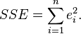
method obtains parameter estimates that minimize the sum of squared
residuals,
SSE,[20][21] also sometimes
denoted RSS:
,
and the true value of the dependent variable,
.
One method of estimation is ordinary least
squares. This
method obtains parameter estimates that minimize the sum of squared
residuals,
SSE,[20][21] also sometimes
denoted RSS:
Minimization of this function results in a set of normal
equations,
a set of simultaneous linear equations in the parameters, which are
solved to yield the parameter estimators,  .
.
In the case of simple regression, the formulas for the least squares estimates are

where
 is the mean (average) of the
 values and
 is the mean of the
 values.
Under the assumption that the population error term has a constant variance, the estimate of that variance is given by:

This is called the mean square error (MSE) of the regression. The denominator is the sample size reduced by the number of model parameters estimated from the same data, (np*) for *p* regressors or (*np1) if an intercept is used.[22] In this case, p=1 so the denominator is n2.
The standard errors of the parameter estimates are given by
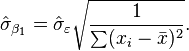
Under the further assumption that the population error term is normally distributed, the researcher can use these estimated standard errors to create confidence intervals and conduct hypothesis tests about the population parameters.
General linear model
For a derivation, see linear least squares
For a numerical example, see linear regression
In the more general multiple regression model, there are p independent variables:

where x~ij~ is the ith observation on the jth independent
variable, and where the first independent variable takes the value 1 for
all i (so
is the regression intercept).
The least squares parameter estimates are obtained from p normal equations. The residual can be written as

The normal equations are

In matrix notation, the normal equations are written as

where the ij element of X is x~ij~, the i element of the column
vector Y is y~i~, and the j element of  is
is  .
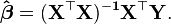
Thus X is n×p, Y is n×1, and
is p×1. The solution is
.
Thus X is n×p, Y is n×1, and
is p×1. The solution is
Diagnostics
See also category: Regression diagnostics
Once a regression model has been constructed, it may be important to confirm the goodness of fit of the model and the statistical significance of the estimated parameters. Commonly used checks of goodness of fit include the Rsquared, analyses of the pattern of residuals and hypothesis testing. Statistical significance can be checked by an Ftest of the overall fit, followed by ttests of individual parameters.
Interpretations of these diagnostic tests rest heavily on the model assumptions. Although examination of the residuals can be used to invalidate a model, the results of a ttest or Ftest are sometimes more difficult to interpret if the model’s assumptions are violated. For example, if the error term does not have a normal distribution, in small samples the estimated parameters will not follow normal distributions and complicate inference. With relatively large samples, however, a central limit theorem can be invoked such that hypothesis testing may proceed using asymptotic approximations.
“Limited dependent” variables
The phrase “limited dependent” is used in econometric statistics for categorical and constrained variables.
The response variable may be noncontinuous (“limited” to lie on some subset of the real line). For binary (zero or one) variables, if analysis proceeds with leastsquares linear regression, the model is called the linear probability model. Nonlinear models for binary dependent variables include the probit and logit model. The multivariate probit model is a standard method of estimating a joint relationship between several binary dependent variables and some independent variables. For categorical variables with more than two values there is the multinomial logit. For ordinal variables with more than two values, there are the ordered logit and ordered probit models. Censored regression models may be used when the dependent variable is only sometimes observed, and Heckman correction type models may be used when the sample is not randomly selected from the population of interest. An alternative to such procedures is linear regression based on polychoric correlation (or polyserial correlations) between the categorical variables. Such procedures differ in the assumptions made about the distribution of the variables in the population. If the variable is positive with low values and represents the repetition of the occurrence of an event, then count models like the Poisson regression or the negative binomial model may be used instead.
Interpolation and extrapolation
Regression models predict a value of the Y variable given known values of the X variables. Prediction within the range of values in the dataset used for modelfitting is known informally as interpolation. Prediction outside this range of the data is known as extrapolation. Performing extrapolation relies strongly on the regression assumptions. The further the extrapolation goes outside the data, the more room there is for the model to fail due to differences between the assumptions and the sample data or the true values.
It is generally advised[citation\ needed] that when performing extrapolation, one should accompany the estimated value of the dependent variable with a prediction interval that represents the uncertainty. Such intervals tend to expand rapidly as the values of the independent variable(s) moved outside the range covered by the observed data.
For such reasons and others, some tend to say that it might be unwise to undertake extrapolation.[23]
However, this does not cover the full set of modelling errors that may be being made: in particular, the assumption of a particular form for the relation between Y and X. A properly conducted regression analysis will include an assessment of how well the assumed form is matched by the observed data, but it can only do so within the range of values of the independent variables actually available. This means that any extrapolation is particularly reliant on the assumptions being made about the structural form of the regression relationship. Bestpractice advice here[citation\ needed] is that a linearinvariables and linearinparameters relationship should not be chosen simply for computational convenience, but that all available knowledge should be deployed in constructing a regression model. If this knowledge includes the fact that the dependent variable cannot go outside a certain range of values, this can be made use of in selecting the model – even if the observed dataset has no values particularly near such bounds. The implications of this step of choosing an appropriate functional form for the regression can be great when extrapolation is considered. At a minimum, it can ensure that any extrapolation arising from a fitted model is “realistic” (or in accord with what is known).
Nonlinear regression
Main article: Nonlinear regression
When the model function is not linear in the parameters, the sum of squares must be minimized by an iterative procedure. This introduces many complications which are summarized in Differences between linear and nonlinear least squares
Power and sample size calculations
There are no generally agreed methods for relating the number of
observations versus the number of independent variables in the model.
One rule of thumb suggested by Good and Hardin is
 ,
where
,
where
 is the sample size,
is the number of independent variables and
is the sample size,
is the number of independent variables and
 is the number of observations needed to reach the desired precision if
the model had only one independent variable.[24] For
example, a researcher is building a linear regression model using a
dataset that contains 1000 patients
().
If he decides that five observations are needed to precisely define a
straight line
(),
then the maximum number of independent variables his model can support
is 4, because
is the number of observations needed to reach the desired precision if
the model had only one independent variable.[24] For
example, a researcher is building a linear regression model using a
dataset that contains 1000 patients
().
If he decides that five observations are needed to precisely define a
straight line
(),
then the maximum number of independent variables his model can support
is 4, because
 .
.
Other methods
Although the parameters of a regression model are usually estimated using the method of least squares, other methods which have been used include:
Bayesian methods, e.g. Bayesian linear regression Percentage regression, for situations where reducing percentage errors is deemed more appropriate.[25] Least absolute deviations, which is more robust in the presence of outliers, leading to quantile regression Nonparametric regression, requires a large number of observations and is computationally intensive Distance metric learning, which is learned by the search of a meaningful distance metric in a given input space.[26]
Software
Main article: List of statistical packages
All major statistical software packages perform least squares regression analysis and inference. Simple linear regression and multiple regression using least squares can be done in some spreadsheet applications and on some calculators. While many statistical software packages can perform various types of nonparametric and robust regression, these methods are less standardized; different software packages implement different methods, and a method with a given name may be implemented differently in different packages. Specialized regression software has been developed for use in fields such as survey analysis and neuroimaging.
Statistics portal
- Curve fitting
- Forecasting
- Fraction of variance unexplained
- Kriging (a linear least squares estimation algorithm)
- Local regression
- Modifiable areal unit problem
- Multivariate adaptive regression splines
- Multivariate normal distribution
- Pearson productmoment correlation coefficient
- Prediction interval
- Robust regression
- Segmented regression
- Stepwise regression
- Trend estimation
References
- Armstrong, J. Scott (2012). “Illusions in Regression Analysis”. International Journal of Forecasting (forthcoming) 28 (3): 689. doi:10.1016/j.ijforecast.2012.02.001.
- David A. Freedman, Statistical Models: Theory and Practice, Cambridge University Press (2005)
- R Dennis Cook; Sanford Weisberg Criticism and Influence Analysis in Regression, Sociological Methodology, Vol. 13. (1982), pp. 313–361
- Legendre_40A.M. Legendre. Nouvelles méthodes pour la détermination des orbites des comètes, Firmin Didot, Paris, 1805. “Sur la Méthode des moindres quarrés” appears as an appendix.
- C.F. Gauss. Theoria Motus Corporum Coelestium in Sectionibus Conicis Solem Ambientum. (1809)
- Gauss2_60C.F. Gauss. Theoria combinationis observationum erroribus minimis obnoxiae. (1821/1823)
- Mogull, Robert G. (2004). SecondSemester Applied Statistics. Kendall/Hunt Publishing Company. p. 59. ISBN 0757511813.
- Galton, Francis (1989). “Kinship and Correlation (reprinted 1989)”. Statistical Science (Institute of Mathematical Statistics) 4 (2): 80–86. doi:10.1214/ss/1177012581. JSTOR 2245330.
- Francis Galton. “Typical laws of heredity”, Nature 15 (1877), 492–495, 512–514, 532–533. (Galton uses the term “reversion” in this paper, which discusses the size of peas.)
- Francis Galton. Presidential address, Section H, Anthropology. (1885) (Galton uses the term “regression” in this paper, which discusses the height of humans.)
- Yule, G. Udny (1897). “On the Theory of Correlation”. Journal of the Royal Statistical Society (Blackwell Publishing) 60 (4): 812–54. doi:10.2307/2979746. JSTOR 2979746.
- Pearson, Karl; Yule, G.U.; Blanchard, Norman; Lee,Alice (1903). “The Law of Ancestral Heredity”. Biometrika (Biometrika Trust) 2 (2): 211–236. doi:10.1093/biomet/2.2.211. JSTOR 2331683. Cite uses deprecated parameters (help)
- Fisher, R.A. (1922). “The goodness of fit of regression formulae, and the distribution of regression coefficients”. Journal of the Royal Statistical Society (Blackwell Publishing) 85 (4): 597–612. doi:10.2307/2341124. JSTOR 2341124.
- Ronald A. Fisher (1954). Statistical Methods for Research Workers (Twelfth ed.). Edinburgh: Oliver and Boyd. ISBN 0050021702.
- Aldrich, John (2005). “Fisher and Regression”. Statistical Science 20 (4): 401–417. doi:10.1214/088342305000000331. JSTOR 20061201.
- Rodney Ramcharan. Regressions: Why Are Economists Obessessed with Them? March 2006. Accessed 20111203.
- N Cressie (1996) Change of Support and the Modiable Areal Unit Problem. Geographical Systems 3:159–180.
- Fotheringham, A. Stewart; Brunsdon, Chris; Charlton, Martin (2002). Geographically weighted regression: the analysis of spatially varying relationships (Reprint ed.). Chichester, England: John Wiley. ISBN 9780471496168.
- Fotheringham, AS; Wong, DWS (1 January 1991). “The modifiable areal unit problem in multivariate statistical analysis”. Environment and Planning A 23 (7): 1025–1044. doi:10.1068/a231025. Cite uses deprecated parameters (help)
- M. H. Kutner, C. J. Nachtsheim, and J. Neter (2004), “Applied Linear Regression Models”, 4th ed., McGrawHill/Irwin, Boston (p. 25)
- N. Ravishankar and D. K. Dey (2002), “A First Course in Linear Model Theory”, Chapman and Hall/CRC, Boca Raton (p. 101)
- Steel, R.G.D, and Torrie, J. H., Principles and Procedures of Statistics with Special Reference to the Biological Sciences., McGraw Hill, 1960, page 288.
- Chiang, C.L, (2003) Statistical methods of analysis, World Scientific. ISBN 9812383107 page 274 section 9.7.4 “interpolation vs extrapolation”
- Good, P. I.; Hardin, J. W. (2009). Common Errors in Statistics (And How to Avoid Them) (3rd ed.). Hoboken, New Jersey: Wiley. p. 211. ISBN 9780470457986.
- Tofallis, C. (2009). “Least Squares Percentage Regression”. Journal of Modern Applied Statistical Methods 7: 526–534. doi:10.2139/ssrn.1406472.
- YangJing Long (2009). “Human age estimation by metric learning for regression problems”. Proc. International Conference on Computer Analysis of Images and Patterns: 74–82.