Article Source

Title: Progressive skyline computation in database systems
Authors: Adrian Colyer

Progressive skyline computation in database systems

Progressive skyline computation in database systems Papadias et al. SIGMOD 2003

I’m still working through some of the papers from SIGMOD 2016 (as some of you spotted, that was the unifying them for last week). But today I’m jumping back to 2003 to provide some context for a streaming analytics paper we’ll be looking at tomorrow. The subject at hand is skyline computation.

Not that sort of skyline.

The skyline operator is important for several applications involving multi-criteria decision making. Given a set of objects p~1~, p~2~, …, p~n~, the operator returns all objects p~i~ such that p~i~ is not dominated by another object p~j~.

A couple of examples help to make the idea much clearer. The running example throughout the paper is a hotels dataset with two attributes per hotel: price and distance from the beach.

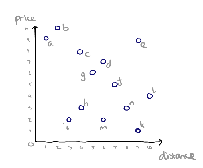
Given some preference or scoring function that is monotone on all attributes (e.g. min) we can compute a skyline. A point p~i~ dominates another point _p~j~ if its coordinate on any axis is not larger than the corresponding coordinate of p~j~.

dominates(h1,h2) :
    (h1.distance < h2.distance) &&
    (h1.price < h2.price)

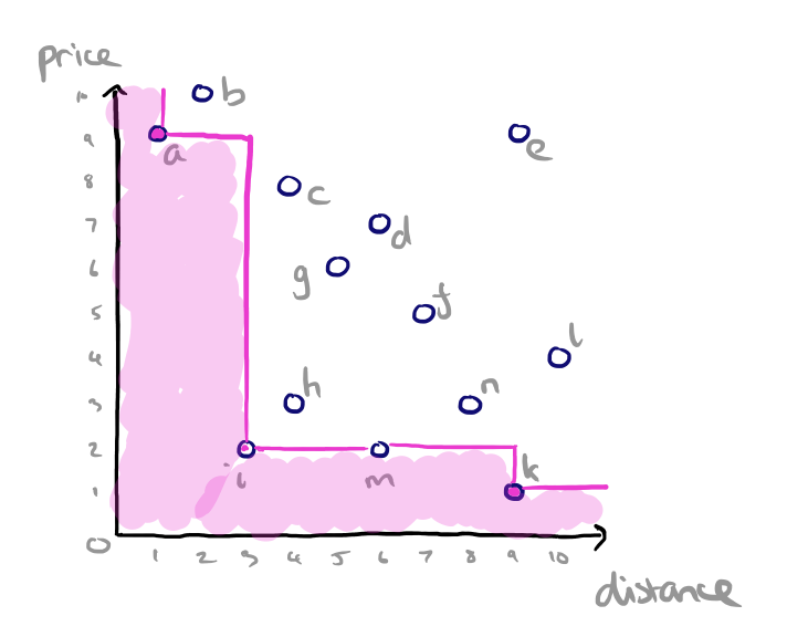
So given two hotels an equal distance from the beach, we prefer the one that is cheaper. And given two hotels that are the same price, we prefer the one closer to the beach. We compute the skyline by finding the points where there is no point that is better on both (all) dimensions, and joining them. The points that define this skyline are a, i, and k.

In a SQL style syntax we might express this query as

SELECT *, FROM Hotels, Skyline OF Price min, Distance min

Here’s another example. Suppose we have a set of data points telling us how well our application performs on a given AWS instance type (for some definition of performance that we can boil down to a single number), and how much that instance type costs. If our scoring function prefers cheaper instance types when performance is equivalent, and instance types that deliver better application performance when cost is equal, then we might draw a skyline that looks like this:

“Progressive skyline computation in database systems” shows us how to efficiently compute a skyline in a database context, as well as introducing a number of variants of the base skyline problem. We also get a review of existing (prior to 2003) algorithms, which I’m going to pass over in favour of explaining the branch-and-bound skyline (BBS) algorithm the authors introduce which outperforms them. A good progressive skyline computation algorithm should have the following qualities:

progressiveness : first results should be reported to the user almost instantly, and the output size should gradually increase
no false misses : eventually the algorithm should generate the entire skyline
_no false hits_: a point should never be reported as a skyline point if it will eventually be replaced (dominated)
_fairness_: the algorithm should not favour points that are particularly good in one dimension
_incorporation of preferences_: the user should be able to specify the order in which skyline points are reported
_universality_: the algorithm should be applicable to any dataset distribution and dimensionality, using some index structure.

The BBS algorithm

BBS is based on a nearest-neighbour search approach, and uses R-trees for data partitioning (though alternative data partitioning data structures would also work).

BBS, similar to the previous algorithms for nearest neighbours and convex hulls, adopts the branch-and-bound paradigm…

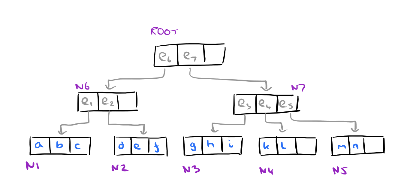
First we need an R-tree for the data. Let’s build one for the hotels data set, with node capacity = 3:

And here are the bounding boxes of the nodes of the R-tree. First the leaves:

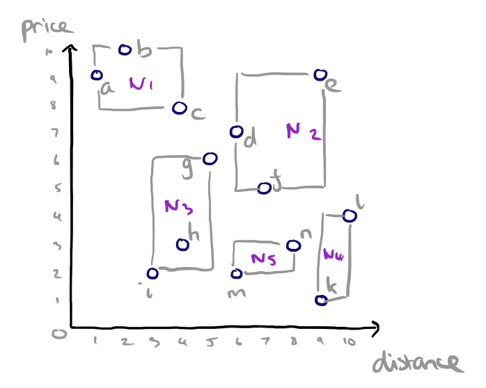
…and then we can draw on the bounding boxes for the intermediate nodes too:

The BBS algorithm starts from the root node of the R-tree, and inserts all of its entries (in this case e6 and e~7~) into a sorted list, ordered by their mindist. That is, sorted by their distance from the the origin.

Distances are computed according to the L~1~ norm, i.e. the mindist of a point equals the sum of its coordinates, and the mindist of a minimum bounding rectangle (i.e. intermediate entry) equals the mindist of its lower-left corner point.

If you’re following along at home, at this stage therefore we have two entries in the list:

e7,4
e6,6

The distance of e7 (which points to N7) is 4 (3+1), and the distance of e6 (which points to N6) is 6 (1+5). We also initialise the set of skyline points, S to the empty set.

While the list is not empty, we repeatedly process the first entry in the list. Starting with e7 therefore, e7 is removed from the list and replaced by its children e3,e4, and e5.

e3, 5
e6, 6
e5, 8
e4, 10

The next step is to process e3:

i, 5
e6, 6
h, 7
e5, 8
e4, 10
g, 11

The top of the list is now i. This is not dominated by any entry in S (which is empty at this point), so we add it to the set S of skyline points. That leaves e6 at the head of the list, and so we expand e6:

h, 7
e5, 8
e1, 9
e4, 10
g, 11

During this expansion, e2 is not added to the list, since it is dominated by an entry in S (namely, i).

At the next step, h7 is discarded since it is dominated by i. That leaves e5 at the head of the list, and it is also discarded since it is dominated by i. Now we expand e1…

a, 10
e4, 10
g, 11
b, 12
c, 12

The top of the list is a, which is not dominated by any member of S, so we add it to S. Expanding e4 we add only k, since l is dominated by i.

k,10
g, 11
b, 12
c, 12

The top of the list is now k, which is added to the skyline set S (S = {i,a,k}). Nodes g, b, and c are then pruned in turn since each is dominated by some member in S. At this point the list is empty and the algorithm is completed.

The pseudo-code for the algorithm is shown below (the paper uses ‘heap’ for what I called a sorted-list).

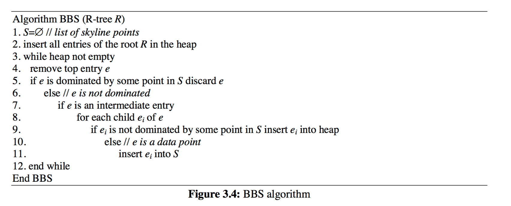
Note that an entry is checked for dominance twice: before it is inserted in the heap, and before it is expanded (processed). The second check is necessary because an entry in the heap may become dominated by some skyline point discovered after its insertion (therefore it does not need to be visited).

The authors show that BBS satisfies all of the criteria given previously, and is I/O optimal meaning the (i) it visits only the nodes that may contain skyline points, and (ii) it does not access the same node twice.

Incremental maintenance

The skyline may change due to subsequent updates (i.e. insertions and deletions) to the database, and hence should be incrementally maintained to avoid recomputation.

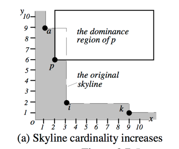
If a new point is dominated by an existing skyline point it is simply discarded. If it is not dominated then it becomes part of a new skyline. BBS performs a window query (on the main-memory R-tree) using dominance region of the new point p, to retrieve any skyline points that may now be obsolete.

The query may return nothing, in which case the skyline simply increases by one point:

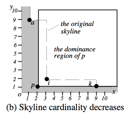
If points are returned though (i and k in the example below), these are removed from the skyline:

Handling deletions is more complex. First, if the point removed is not in the skyline (which can be easily checked by the main-memory R-tree using the point’s coordinates), no further processing is necessary. Otherwise, part of the skyline must be reconstructed…

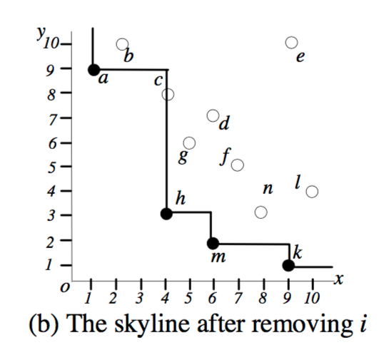
Which part? The part that is exclusively dominated by the skyline point being deleted (i.e. areas not dominated by other skyline points). This corresponds with the shaded area in the example below:

Recomputing this part of the skyline leaves us with:

Variations

A constrained skyline query returns the most interesting data points in a space defined by constraints (e.g. price between x and y). BBS easily processes such queries by simply pruning any entries that do not intersect the constrained region. (This constrained processing method is used during incremental maintenance of a skyline when a skyline point is deleted).

A ranked skyline (top-K) skyline query returns the top K skyline points according to some user provided input function – which must be monotone on each attribute. BBS handles such queries by replacing the mindist function with the user provided function, and terminating after exactly K points have been reported. mindist is essentially the special case where the preference function is pref(x,y) = x + y.

A grouped-by skyline query returns multiple skylines, one for each group (e.g., skylines for 3-star, 4-star, and 5-star hotels). BBS can be adapted for this by keeping a separate in-memory R-tree for each class, together with a single heap containing all the visited entries.

A dynamic skyline query provides dimension functions and returns a skyline in the data space defined by the outputs of those functions. A example makes this clearer, suppose we have the user’s current location, and a database with hotel locations. We could then compute a dimension which is ‘distance from user’ and produce a skyline based on this. BBS can be used for dynamic skylines simply by computing mindist in the dynamic space.

An enumerating query returns for each skyline point p, the number of points dominated by p. A K-dominating query retrieves the K points that dominate the largest number of other points (strictly speaking, this is not a skyline query, since the result does not necessarily contain skyline points).

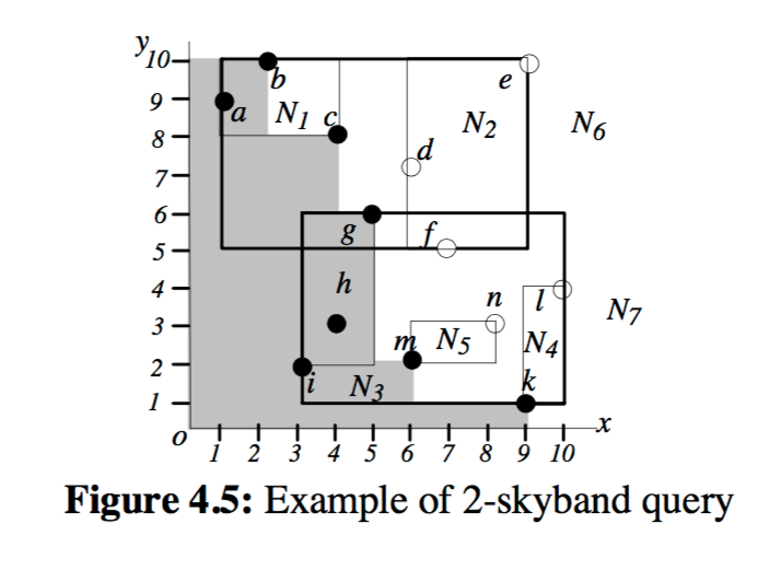
A K-skyband query reports the set of points that are dominated by at most K points.

Conceptually, K represents the thickness of the skyline; the case that K=0 corresponds to a conventional skyline.

Using the hotels example, here’s what the result of a 2-skyband query would look like.

Approximate skylines can be created from a histogram on the dataset, or progressively following the root visit in BBS. See section 5 of the paper for details.

Stop Thinking, Just Do!