Article Source

• Title: Deep Learning in a Nutshell: Reinforcement Learning
• Authors: Tim Dettmers

---

Deep Learning in a Nutshell: Reinforcement Learning

This post is Part 4 of the Deep Learning in a Nutshell series, in which I’ll dive into reinforcement learning, a type of machine learning in which agents take actions in an environment aimed at maximizing their cumulative reward.

Deep Learning in a Nutshell posts offer a high-level overview of essential concepts in deep learning. The posts aim to provide an understanding of each concept rather than its mathematical and theoretical details. While mathematical terminology is sometimes necessary and can further understanding, these posts use analogies and images whenever possible to provide easily digestible bits that make up an intuitive overview of the field of deep learning. Previous posts coveredcore concepts in deep learning, training of deep learning networks and their history, andsequence learning.

Reinforcement Learning

Learning to ride a bike requires trial and error, much like reinforcement learning. (Video courtesy of Mark Harris, who says he is “learning reinforcement” as a parent.)

Remember how you learned to ride a bike? More than likely an adult stood or walked behind you and encouraged you to make the first moves on your bike­­, and helped you get going again when you stumbled or fell. But it is very difficult to explain to a child how to ride a bike, and even a good explanation makes little sense to someone who has never ridden before: you have to get the feel for it. So how did you learn to ride a bike if it could not be clearly explained? Well, you just tried to ride the bike, and more than likely you fell, or at least stopped abruptly and had to catch yourself. You fell or stumbled repeatedly—until you got some little spark of success after riding for a few meters before you fell again.

During this learning process, the feedback signals that tell us how well we do are either pain: “Ouch! I fell! That hurts! I will avoid doing what led to this next time!”, or reward: “Wow! I am riding the bike! This feels great! I just need to keep doing what I am doing right now!”

In a reinforcement learning problem, we take the view of an agent that tries to maximize the reward that it is receiving from making decisions. Thus an agent that receives the maximum possible reward can be viewed as performing the best action for a given state. An agent here refers to an abstract entity which can be any kind of object or subject that performs actions: autonomous cars, robots, humans, customer support chat bots, go players. The state of an agent refers to the agent’s position and state of being in it’s abstract environment; for example, a certain position in a virtual reality world, a building, a chess board, or the position and speed on a racetrack.

To simplify the problem and the solution of a reinforcement problem, the environment is often simplified so that the agent only knows about the details which are important for decision making while the rest is discarded. Just like in the bike riding example, the reinforcement algorithm has only two sources of feedback to learn from: penalty (pain of falling) and reward (thrill of riding for a few meters). If we view penalty as negative reward, then the whole learning problem concerns exploring an environment and trying to maximize the reward that our agent receives for passing from state to state until a goal state is reached (driving autonomously from A to B; winning a chess game; solving a customer problem via chat): this is reinforcement learning in a nutshell.

The Value Function

Reinforcement learning is about positive and negative rewards (punishment or pain) and learning to choose the actions which yield the best cumulative reward. To find these actions, it’s useful to first think about the most valuable states in our current environment. For example, on a racetrack the finish line is the most valuable, that is the state which is most rewarding, and the states which are on the racetrack are more valuable than states that are off-track.

Once we have determined which states are valuable we can assign “rewards” to various states. For example, negative rewards for all states where the car’s position is off-track; a positive reward for completing a lap; a positive reward when the car beats its current best lap time; and so on. We can imagine the states and rewards as a discrete function. For example a racetrack could be represented by a grid of 1-by-1 meter tiles. The rewards on a tile are represented by numbers. For example the goals might have reward 10, and the tiles which are off track have a reward of -2 while all other tiles have a reward of 0. If we picture this function in 3 dimensions, then we we could imagine that the best action is to stay as high as possible (maximize reward).

For each of these states there are intermediate states which are not necessarily rewarding (reward 0) but are necessary milestones on the path towards a reward. For example, you need to pass the first turn on a racetrack in order to finish a lap, and you need to finish a lap before you can improve your lap time.

The trained or fitted value function assigns partial rewards to the intermediate states so that, for example, completing the second turn is more valuable than the first because the second turn represents a state which is closer to the next goal. The value function helps the agent make good decisions by providing intermediate rewards that make it easier for the agent to choose which state to go to next, given the current state.

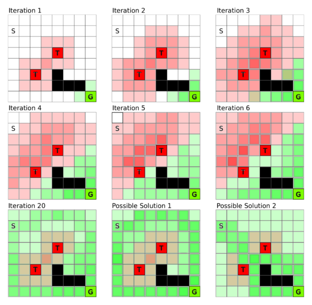
Figure 1: Value iteration constructs the value function over all states over time. Here each square is a state: S is the start state, G the goal state, T squares are traps, and black squares cannot be entered. In value iteration we initialize the rewards (traps and goal state) and then these reward values spread over time until an equilibrium is reached. Depending on the penalty value on traps and the reward value for the goal different solution patterns might emerge; the last two grids show such solution states.

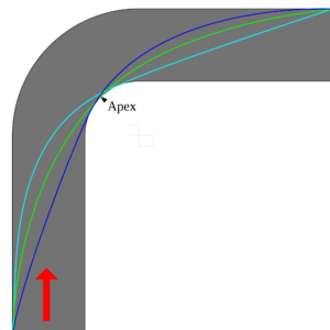
Figure 2: Different racing lines around a corner. Each racing line has a different distance, range of possible speeds, and force exerted on the tires. A value function optimizing for lap time will optimize this problem to find state transitions which minimize the total time spent in the turn. Image source

This framework means that each given state’s value is influenced by all the values of the states which are easily accessible from that state. Figure 1 shows an example world where each square is a state and S and G are the start and goal states, respectively, T squares are traps, and black squares are states which cannot be entered (big boulders blocking the way). The goal is to move from state S to state G. If we imagine this to be our racetrack, then over time we create a “ramp” from the start state to the goal state, so that we just have to go along the direction which is steepest in order to find the goal. This is the main goal of the value function: to provide an estimate of the value of each state, so that we can make step-by-step decisions which lead to a reward.

The value function can also capture the subtleties of a problem. For example, the reward for maintaining a large distance from the sides of a racetrack is less negative because this state is farther from the states which are designated off-track; but at the same time it is not efficient to drive in the middle of the track to achieve a good lap time (the car cannot take turns at high velocity). So safety and speed compete against each other and the value function finds the most suitable fast-yet-safe path on the track. The final solution can be tuned by altering the reward values. For example if a fast lap time gives a high reward, the value function will assign larger values to states which are more risky but allow faster lap times.

Discounting Factor

Even though the value function handles competing rewards, it also depends on a parameter called the discounting factor that defines its exact behavior by limiting how much an agent is affected by rewards which lie in the far future. This is done by multiplying the partial reward by the discounting factor whenever a state change is made. So with a discounting factor of 0.5, the original reward will be one eighth of its value after only 3 state changes, causing the agent to pursue rewards in close proximity rather than rewards which are further away. Thus the discounting factor is a weight that controls whether the value function favors prudent or greedy actions.

For example, a race car might get high reward by going fast, so a very greedy decision with discount factor close to zero might always go as fast as possible. But a more prudent agent knows that going as fast as possible is a bad idea when there is a sharp turn ahead, while slowing down at the right moment may yield a better lap time later, and thus a higher reward. To have this foresight, the agent needs to receive the reward for going faster later, so a discounting factor closer to 1 may be better.

The value function’s discounting factor ensures that rewards that are far away diminish proportionally to the distance or steps it takes to reach them. This factor is usually set to a value which values long-term rewards highly, but not too high (for example the reward decays by 5% per state transition).

The algorithm learns the specific partial reward value of each state of the value function by first initializing all states to zero or their specific reward value, and then searching all states and all their possible next states and evaluating the reward it would get in the next states. If it gets a (partial) reward in the next state, it increases the reward of the current state. This process repeats until the partial reward within each state doesn’t change any more, which means that it has taken into account all possible directions to find all possible rewards from all possible states. You can see the process of this value iteration algorithm in Figure 1.

This may seem inefficient at first, but a trick associated with dynamic programming makes it much more efficient. Dynamic programming solves higher-order problems in terms of already solved sub-problems: the computed reward for going from state B to C can be reused in computing the rewards for state chains A->B->C and D->B->C.

In summary, the value function and value iteration provide a map of partial rewards which guides the agent toward rewarding states.

The Policy Function

The policy function represents a strategy that, given the value function, selects the action believed to yield the highest (long-term) reward. Often there is no clear winner among the possible next actions. For example, the agent might have the choice to enter one of four possible next states A,B,C, and D with reward values A=10, B=10, C=5 and D=5. So both A and B would be good immediate choices, but a long way down the road action A might actually have been better than B, or action C might even have been the best choice. It is worth exploring these options during training, but at the same time the immediate reward values should guide the choice. So how can we find a balance between exploiting high reward values and exploring less rewarding paths which might return high rewards in the long term?

A clever way to proceed is to take choices with probability proportional to their reward. In this example the probability of taking A would be 33% (10/(10+10+5+5)), and the probability of taking B, C, and D would be 33%, 16%, and 16%, respectively. This random choice nature of the policy function is important to learning a good policy. There might exist effective or even essential strategies that are counter-intuitive but necessary for success.

For example, if you train a race car to go fast on a racetrack it will try to cut the corners with the highest speed possible. However, this strategy will not be optimal if you add competitors into the mix. The agent then needs to take into account these competitors and might want to take turns slower to avoid the possibility of a competitor overtaking or worse, a collision. Another scenario might be that cornering at very high speed will wear the tires much quicker resulting in the need for a pit-stop, costing valuable time.

Note that the policy and value functions depend on each other. Given a certain value function, different policies may result in different choices, and given a certain policy, the agent may value actions differently. Given the policy “just win the game” for a chess game, the value function will assign high value to the moves in the game which have high probability of winning (sacrificing chess pieces in order to win safely would be valued highly). But given the policy “win with a large lead or not at all”, then the policy function will just learn to select the moves which maximize the score in the particular game (never sacrifice chess pieces).

These are just two examples of many. If we want to have a specific outcome we can use both the policy and value functions to guide the agent to learn good strategies to achieve that outcome. This makes reinforcement learning versatile and powerful.

We train the policy function by (1) initializing it randomly—for example, let each state be chosen with probability proportional to its reward—and initialize the value function with the rewards; that is, set the reward of all states to zero where no direct reward is defined (for example the racetrack goal has a reward of 10, off-track states have a penalty of -2, and all states on the racetrack itself have zero reward). Then (2) train the value function until convergence (see Figure 1), and (3) increase the probability of the action (moving from A to B) for a given state (state A) which most increases the reward (going from A to C might have a low or even negative reward value, like sacrificing a chess piece, but it might be in line with the policy of winning the game). Finally, (4) repeat from step (1) until the policy no longer changes.

The Q-function

We’ve seen that the policy and value functions are highly interdependent: our policy is determined mostly by what we value, and what we value determines our actions. So maybe we could combine the value and policy functions? We can, and the combination is called the Q-function.

The Q-function takes both the current state (like the value function) and the next action (like the policy function) and returns the partial reward for the state-action pair. For more complex use cases the Q-function may also take more states to predict the next state. For example if the direction of movement is important one needs at least 2 states to predict the next state, since it is often not possible to infer precise direction from a single state (e.g. a still image). We can also just pass input states to the Q-function to get a partial reward value for each possible action. From this we can (for example) randomly choose our next action with probability proportional to the partial reward (exploration), or just take the highest-valued action (exploitation).

However, the main point of the Q-function is actually different. Consider an autonomous car: there are so many “states” that it is impossible to create a value function for them all; it would take too long to compute all partial rewards for every possible speed and position on all the roads that exist in on Earth. Instead, the Q-function (1) looks at all possible next states that lie one step ahead and (2) looks at the best possible action from the current state to that next state. So for each next state the Q-function has a look-ahead of one step (not all possible steps until termination, like the value function). These look-aheads are represented as state-action pairs. For example, state A might have 4 possible actions, so that we have the action pairs A->A, A->B, A->C, A->D. With four actions for every state and a 10×10 grid of states we can represent the entire Q-function as four 10×10 matrices, or one 10x10x4 tensor. See Figure 3 for a Q-function which represents the solution to a grid world problem (a 2D world where you can move to neighboring states) where the goal is located in the bottom right corner.

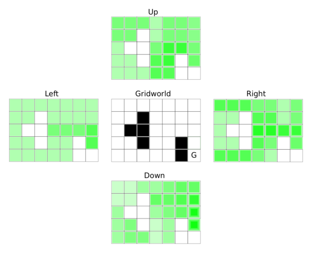
Figure 3: Q-function for a grid world problem with blocking states (black), where the goal is the bottom right corner. The four matrices show the reward (or Q-values of the Q-function) for all four actions in each state, where a darker green indicates a higher Q-value. An agent will choose darker states with higher probability, or in the greedy case will always choose the action which has the highest surrounding Q-value. This will guide the agent as quickly as possible to the goal. This behavior is independent of the starting position.

In some cases we need to model sheer infinite states. For example, in an autonomous car the “state” is often represented as a continuous function such as a neural network, which just takes all the state variables, such as speed and position of the car, and outputs Q-values for each action.

Why does it help to have information about only some states? Many states are very well correlated, so the same action taken at two different, but similar, states may lead to success in both cases. For example, every turn on a racetrack will be different, but the things that you learn from each left turn—when to start a turn, how speed should be adjusted, etc.—are valuable for the next left turn. So over time, a car-driving agent can learn to make better and better left turns, even on tracks it has never seen.

Q-Learning

To train the Q-function we initialize all Q-values of all state-action pairs to zero and initialize the states with their given rewards. Because the agent does not know how to get to the rewards (an agent can only see the Q-value of the next states, which will all be zero) the agent may go through many states until it finds a reward. Thus we often terminate training the Q-function after a certain length (for example, 100 actions) or after a certain state has been reached (one lap on a racetrack). This ensures we don’t get stuck in the process of learning good actions for one state since it’s possible to be stuck in a hopeless state where you can make as many iterations as you like and never receive any noticeable rewards.

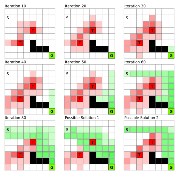
Figure 4: Q-learning in a grid world, where S is the start state, G the goal state, T squares are traps, and black squares are blocked states. During Q-learning the agent explores the environment step by step and does not find the goal state G initially. Once a chain is built from the goal state to the proximity of the start state the algorithm quickly converges to a solution which it then further adapts to find the best strategy for the problem.

Learning the Q-function proceeds from end (the reward) to start (the first state). Figure 4 depicts the grid world example from Figure 1 in terms of Q-learning. Assume the goal is to reach the goal state G in the smallest number of steps. Initially the agent makes random moves until it (accidentally) reaches either a trap or the goal state. Because the traps are closer to the start state the agent is most likely to hit a trap first, but this pattern is broken once the agent stumbles upon the goal state. From that iteration on the states right before the goal state (one step look-ahead) have a partial reward and since the reward is now closer to the start the agent is more likely to hit such a rewarding state. In this way a chain of partial rewards builds up more quickly the more often the agent reaches a partial reward state so that the chain of partial rewards from goal to start state is quickly completed (see Figure 4).

Deep Q-learning

An autonomous vehicle may need to consider many states: every different combination of speed and position is a different state. But most states are similar. Is it possible to combine similar states so that they have similar Q-values? Here is where deep learning comes into play.

We can input the current point of view of the driver—an image—into a convolutional neural network (CNN) trained to predict the rewards for the next possible actions. Because images for similar states are similar (many left turns look similar) they will also have similar actions. For example, a neural network will be able to generalize for many left turns on a racetrack and even make appropriate actions for left turns that were not encountered before. Just like a CNN trained on many different objects in images can learn to correctly distinguish these objects, a network trained on many similar variations of left turns will be able to make fine adjustments of speed and position for each different left turn it is presented.

To use deep Q-learning successfully, however, we cannot simply apply the rule to train the Q-function described previously. If we apply the Q-learning rule blindly, then the network will learn to do good left turns while doing left turns, but will start forgetting how to do good right turns at the same time. This is so because all actions of the neural network use the same weights; tuning the weights for left turns makes them worse for other situations. The solution is to store all the input images and the output actions as “experiences”: that is, store the state, action and reward together.

After running the training algorithm for a while, we choose a random selection from all the experiences gathered so far and create an average update for neural network weights which maximizes Q-values (rewards) for all actions taken during those experiences. This way we can teach our neural network to do left and right turns at the same time. Since very early experiences of driving on a racetrack are not important—because they come from a time where our agent was less experienced, or even a beginner—we only keep track of a fixed number of past experiences and forget the rest. This process is termed experience replay.

The following video shows the Deep Q-learning algorithm learning to play Breakout at an expert level. (Thanks to Károly Zsolnai-Fehér’s for permission for embedding this video. You may be interested in his 2-minute paper youtube channel, where he explains important scientific work in plain language in just two minutes.)

Experience replay is a method inspired by biology. The hippocampus in the human brain is a reinforcement learning center in each hemisphere of the brain. The hippocampus stores all the experiences that we make during the day but it has a limited memory capacity for experiences and once this capacity is reached learning becomes much more difficult (cramming too much before an exam). During the night this memory buffer in the hippocampus is emptied into the cortex by neural activity that spreads across the cortex. The cortex is the “hard drive” of the brain where almost all memories are stored. Memories for hand movements are stored in the “hand area”, memories for hearing are stored in the “hearing area”, and so on. This characteristic neural activity that spreads outward from the hippocampus is termed sleep spindle. While there is currently no strong evidence to support it, many sleep researchers believe that we dream to help the hippocampus to integrate the experiences gathered over the day with our memories in the cortex to form coherent pictures.

So you see that storing memories and writing them back in a somewhat coordinated fashion is an important process not only for deep reinforcement learning but also for human learning. This biological similarity gives us a little confidence boost that our theories of the brain might be correct and also that the algorithms we design are on the right path towards intelligence.

AlphaGo

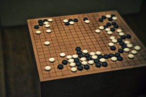
(Image: Linh Nguyen/Flickr)

AlphaGo, developed by Google DeepMind, made big news in 2016 by becoming the first computer program to beat a human professional player at the game of Go. It then went on to beat Lee Sedol, one of the top Go players in the world, four games to one. AlphaGo combines many of the elements mentioned previously in this post; namely (1) value and (2) policy neural networks which represent (1) the value function over the current configuration in a go game, and therefore predicts the relative value of one move over another, and (2) the policy function which suggests what moves should be picked in order to win the game. These networks are convolutional networks, which treat the Go board as a 19×19 input “image” (one pixel for each position).

Because we already have many recorded Go games, it is useful to train the policy network by using existing Go game data played by professionals. The policy network is trained on this data to predict the next move that Go champions played in their games given a certain game configuration.

Once this supervised training phase is finished, reinforcement learning comes into play. Here AlphaGo plays against itself and tries to refine its strategy to pick moves (policy network) and its strategy to evaluate who is winning (value network). Even just training the policy network is a significantly better approach than the previous best-known Go algorithm, called Pachi, which makes use of tree-search algorithms and heuristics. However, one can still improve the the performance of the deep learning approach significantly with the help of the value network.

The value network tends to generalize poorly when it is trained on whole games, because configurations are highly correlated so that the network learns to identify a game (this is game A vs. B from Beijing, 1978, so I know A wins) rather than identifying good moves. To circumvent this problem, DeepMind generated a lot of data by letting AlphaGo play against itself and then taking a few positions of each game to train the value network. This is similar to experience replay, where we never look at lengthy action sequences in isolation, but rather at combinations of very different states and actions.

The value network showed similar performance to Monte Carlo search trees with rollout policy, but AlphaGo used Monte Carlo search trees on top of the deep learning approach for even better performance. What are Monte Carlo search trees with rollout policy? Imagine a tree of game configurations where a move is an edge and nodes are different game configurations. For example, you are in a certain game configuration and you have 200 possible moves—that is, there are 200 nodes connected to your current node—and then you choose a certain move (an edge leading to a node) resulting in a new tree with 199 different nodes which can be reached after the current move. This tree, however, is never fully expanded since it grows exponentially and would take far too long to evaluate the tree completely, so in a Monte Carlo tree search we only take a route along the tree to a certain depth to make evaluation more efficient.

In the rollout policy, we look at the current state, apply the policy network to select a move to the next node in the tree and repeat for all following moves for both players until the game ends and a winner is found. This provides another quick and greedy way to estimate the value of a move. This insight can then also be used to improve value network accuracy. With a more accurate value function we are also able to improve our policy function further: knowing with greater accuracy whether a move is good or bad lets us develop strategies based on good moves which were previously thought to be bad. Or in other words, AlphaGo is able to consider strategies which are unthinkable for humans to work, but they actually win games.

AlphaGo also uses Monte Carlo search trees for training. The trees contain edges of Q values, visit counts (N), and a prior probability (P) which are updated at each iteration. Initially, the Q-value, visit count and prior probability are zero. During an iteration, an action is selected according to the three parameters (Q,N,P). For example, to decide if it is a good move to play a stone on position E5 the new state of the board for this move is evaluated by a combination of (1) the policy network, which sets the initial prior probability for that move, (2a) the value network which assigns a value to the move, and (2b) Monte Carlo rollout which assigns another value to the move. Steps (2a) and (2b) are weighted by a parameter and the Q-values and visit counts (N) are updated with the mean evaluations on that path (increase the Q value if the move was relatively good on average, decrease otherwise). With every iteration the value for the same move is reduced slightly by the visit count, so that new moves will be explored with higher probability. This ensures a balance of exploration and exploitation. However, we also get more and more accurate estimates for moves that we already played. The tree assigns higher Q-values to very strong moves over time. Through this training procedure AlphaGo learns to play better moves with every training iteration and thus learns which moves will win the game. From here the rest is just computing power and time until we create a Go bot which is better than human professionals.

Conclusion

In this post we’ve seen that reinforcement learning is a general framework for training agents to exhibit very complex behavior. We looked at the constituents of reinforcement learning including the value and policy functions and built on them to reach deep reinforcement learning. Deep reinforcement learning holds the promise of a very generalized learning procedure which can learn useful behavior with very little feedback. It is an exciting but also challenging area which will certainly be an important part of the artificial intelligence landscape of tomorrow. You may also be interested in the Train Your Reinforcement Learning Agents at the OpenAI Gym.

If you would like to read the rest of the series, check out part 1: core concepts in deep learning, part 2: training of deep learning networks and their history, and part 3: sequence learning. I hope you enjoy this series!

If you have questions, please ask in the comments below and I will answer.

Acknowledgments

I want to thank Mark Harris for helping me to polish this blog post series with his thoughtful editing and helpful suggestions. I also want to thank Alison Lowndes and Stephen Jones for making this series possible.