Article Source

Title: Notes on Graph Theory

Notes on Graph Theory

[PDF version: Notes on Graph Theory – Logan Thrasher Collins]

Definitions [1]

General Properties 1.1

1.1.1 Order: number of vertices in a graph.
1.1.2 Size: number of edges in a graph.
1.1.3 Trivial graph: a graph with exactly one vertex.
1.1.4 Nontrivial graph: a graph with an order of at least two.
1.1.5 Neighboring vertices: if e=uv is an edge of G, then u and v are joined by e and are neighbors. They are also called incident with each other.
1.1.6 Complete graph: a graph with the maximum possible size for a graph of order n. For a complete graph, every pair of vertices is adjacent.

Subgraphs 1.2

1.2.1 Subgraph: consider a graph G, a subset of its vertices V(H)⊆V(G), and a subset of its edges E(H)⊆E(G). The graph H is a subgraph of G.
1.2.2 Proper subgraph: consider a subgraph H⊆G. If G contains at least one vertex or edge not in H, then H is a proper subgraph of G.
1.2.3 Spanning subgraph: a subgraph H⊆G with the same vertex set as G.
1.2.4 Induced subgraph: a subgraph H⊆G which possesses the same edges as G, but only for the vertices V(H)⊆V(G), which might not be the full vertex set of the graph G.
1.2.5 Clique: a subgraph H⊆G for which H is also a complete graph.

Traversing Graphs 1.3

1.3.1 Walk: a sequence of vertices starting with u∈G and ending with v∈G such that consecutive vertices are adjacent.
1.3.2 Closed walk: a walk for which u=v.
1.3.3 Open walk: a walk for which u≠v.
1.3.4 Length of a walk: the number of edges traversed in a walk.
1.3.5 Trivial walk: a walk with a length of zero.
1.3.6 Trail: a walk in which no edge is traversed more than once.
1.3.7 Path: a walk in which no vertex is traversed more than once.
1.3.8 Circuit: a closed trail with length L≥3.
1.3.9 Cycle: a circuit which does not repeat any vertices except for the first and last. An odd cycle is a cycle with an odd length, an even cycle is a cycle with an even length, and a k-cycle is a cycle of length k.
1.3.10 Distance: given vertices u and v, the distance d(u,v) is the smallest length of any u-v path in G. This path is called a geodesic.
1.3.11 Diameter: the diameter diam(G) is the greatest distance between any pair of vertices in the connected graph G.
3.12 Face: a space enclosed by a cycle. The space outside of a graph is also defined as a face.

Connectedness 1.4

1.4.1 Connected vertices: if G contains a path from vertex u to vertex v, then u and v are connected vertices.
1.4.2 Connected graph: a graph for which every pair of vertices is connected.
1.4.3 Disconnected graph: a graph which is not a connected graph.
1.4.4 Component: a connected subgraph of G which is not a proper subgraph of any other subgraph of G. Alternatively, this is a connected subgraph H⊆G (connected within itself) which is not connected to any other subgraph in G.

Common Types of Graphs 1.5

1.5.1 Empty graph: a graph with n vertices and no edges.

Fig.1

1.5.2 Bipartite graph: a graph for which the vertex sets of G can be partitioned into two subsets U and W (called partite sets), such that every edge connects a vertex of U to a vertex of W. Note that this does not mean every vertex of U is adjacent to a vertex of W.
1.5.3 Complete bipartite graph: a bipartite graph for which vertex of U is adjacent to a vertex of W. This type of graph is denoted as K~s,t~, where s and t represent the number of vertices in the sets U and W respectively.
1.5.4 Star: a complete bipartite graph for which either s=1 or t=1.
1.5.5 Multipartite graph: a graph for which V(G) can be partitioned into k subsets such that, for every edge uv∈G, the vertices u and v belong to different partite sets. This does not mean that every vertex of a given partite set is adjacent to a vertex from another partite set. Multipartite graphs are also called k-partite graphs.
1.5.6 Complete multipartite graph: a multipartite graph for which every vertex of a given partite set of the graph is adjacent to a vertex of another partite set of the graph.
1.5.7 Multigraph: in a multigraph, more than one edge is allowed between any given pair of vertices (multi-edges).
1.5.8 Pseudograph: a multigraph which allows one or more edges which joins a given vertex to itself (a loop or self-edge).
1.5.9 Weighted graph: a multigraph in which all multi-edges are replaced by single edges equipped with weights. The values of the weights are defined as the number of multi-edges between a given pair of vertices.
1.5.10 Digraph: a set of vertices together with a set of edges defined by ordered pairs of vertices (called directed edges or arcs). Given a directed edge (u,v), the vertex u is called adjacent to v and the vertex v is called adjacent from u. The vertices u and v are also said to be incident with the directed edge (u,v).
1.5.11 Oriented graph: a digraph without any pairs of vertices u and v connected by an equal number of edges with opposite directions.
1.5.12 Simple Graph: an undirected graph with no self-edges.

Operations on Graphs 1.6

1.6.1 Complement: a graph’s complement Ḡ possesses the same vertices as G, but has an edge uv if and only if uv is not an edge of G.
1.6.2 Union: given two graphs G and A, their union G∪A creates a disconnected graph

Fig.2

with a vertex set V(G)∪V(A) and an edge set V(G)∪V(A).

1.6.3 Join: given two graph G and A, their join G+A creates the union of the graphs with the added property that each vertex of G is adjacent to all the vertices of A and each vertex of A is adjacent to all the vertices of G (as such, G+A is a connected graph).
1.6.4 Cartesian product: given two graphs G and A, their Cartesian product G⨯A has a vertex set for which every vertex of G⨯A is an ordered pair (u,v) where u∈V(G) and v∈V(A). Two distinct vertices (u,v) and (s,t) within G⨯A are adjacent if either u=s and vt∈E(H) or v=t and us∈E(G). Note that this method of constructing G⨯A requires

Fig.3

the vertices of G and A to be labeled in a sequential manner (i.e. V(G)={g~1~,g~2~,…,g~n~} and V(A)={a~1~,a~2~,…,a~m~}) so that equivalences between vertices can be decided. In addition, the Cartesian product of graphs is commutative, that is G⨯A=A⨯G.

1.6.5 Transpose: given a digraph D, its transpose is the digraph R such that the direction of each arc in D is reversed.

Definitions [2]

Degrees 2.1

2.1.1 Degree: the number of edges incident with a vertex v. This is equivalent to the number of vertices adjacent to v. The degree of v is often denoted as deg(v).
2.1.2 Neighborhood: the set N(v) of vertices adjacent to a vertex v.
2.1.3 Isolated vertex: a vertex with a degree of zero.
2.1.4 Leaf: a vertex with a degree of one, also called an end-vertex.
2.1.5 Minimum degree: given a graph G, its minimum degree δ(G) is the lowest degree among the vertices of G.
2.1.6 Maximum degree: given a graph G, its maximum degree Δ(G) is the highest degree among the vertices of G.
2.1.7 Even vertex: a vertex of even degree.
2.1.8 Odd vertex: a vertex of odd degree.
2.1.9 Outdegree: for a digraph D, the outdegree od(v) is the number of vertices of D to which v is adjacent.
2.1.10 Indegree: for a digraph D, the indegree id(v) is the number of vertices of D from which v is adjacent.
2.1.11 Regular graph: a graph with δ(G)=Δ(G) is called regular. For regular graphs, all vertices have the same degree. The degree r of a regular graph’s vertices is used to classify the graph as r-regular.
2.1.12 Cubic graph: a graph which is 3-regular.
2.1.13 Degree sequence: any list of the degrees found in some graph. Usually, degree sequences can be ordered in multiple ways.
2.1.14 Graphical: a finite sequence of nonnegative integers is called graphical if it corresponds to some graph G.

Irregular Graphs 2.2

2.2.1 Irregular graph: a graph G with an order of at least two is called irregular if every pair of vertices u∈V(G) and v∈V(G) have distinct degrees.

Fig.4

2.2.2 F-degree: for a nontrivial subgraph F⊆G and a vertex v∈G, the F-degree (denoted Fdeg) is the number of copies of F in G which contain v.
2.2.3 F-regular: a graph is F-regular if every pair of vertices has the same F-degree.
2.2.4 F-irregular: a graph is F-irregular if all pairs of vertices have distinct F-degrees.
2.2.5 Underlying graph: if all multi-edges in a multigraph M are replaced by single edges, the resulting graph is called the underlying graph of M.

Matrices and Edge Lists for Graphs 2.3

2.3.1 Adjacency matrix: given a graph G of order n, its adjacency matrix A=a~ij~ is the n x n matrix defined below. Adjacency matrices of simple graphs are symmetric with zeros along the diagonal. Adjacency matrices of pseudographs may have some ones on the diagonal (which indicates self-edges). Adjacency matrices of multigraphs may have integer values greater than one (which indicate more than one edge between given pairs of vertices). Adjacency matrices of digraphs (specifically oriented graphs) are not symmetric (indicating directed edges).

Eq.1

2.3.2 Incidence matrix: given a graph G of order n and size m, its incidence matrix B=b~ij~ is the n x m matrix defined below.

Eq.2

2.3.3 Edge list: a list of ordered pairs (u~1~,v~1~), (u~2~,v~2~), … , (u~n~,u~n~) which corresponds to all of the edges in a graph.

Definitions [3]

Isomorphic Graphs 3.1

3.1.1 Equal graphs: a pair of graphs with the same vertex set and edge set.
3.1.2 Isomorphic graphs: two graphs G and H are isomorphic if there exists a bijective function ϕ which maps V(G) to V(H) such that uv∈E(G) if and only if ϕ(u)ϕ(v)∈V(H). The bijective function ϕ is called an isomorphism. Isomorphic graphs are denoted as G≌H. Isomorphisms are also equivalence relations (and so possess the properties of equivalence relations). Note that isomorphic graphs possess the same structure, but might be drawn differently.
3.1.3 Isomorphic digraphs: digraphs D~1~ and D~2~ are isomorphic if there exists a bijective function ϕ which maps V(D~1~) to V(D~2~) such that the directed edge (u~1~,v~1~)∈E(D~1~) if and only if (ϕ(u~1~),ϕ(v~1~))∈E(D~2~).
3.1.4 Isomorphic to a subgraph: given unlabeled graphs G and H, if for any labeling of

Fig.5

the vertices of H and G, the labeled graph H is isomorphic to a subgraph of the labeled graph G.

3.1.5 Non-isomorphic graphs: graphs that are not isomorphic, denoted as G≇H.
3.1.6 Self-complementary: a graph G which is isomorphic with its complement Ḡ.

Trees 3.2

3.2.1 Bridge: consider an edge e=uv of a connected graph G. If removing e from G gives a disconnected graph, then e is a bridge.
3.2.2 Acyclic graph: a graph with no cycles. If an acyclic graph consists of more than one component, it is also called a forest.
3.2.3 Tree: an acyclic connected graph T.
3.2.4 End-vertex: a vertex with a degree of one.
3.2.5 Double star: a tree containing exactly two vertices that are not end-vertices.
3.2.6 Linear graph: a tree with exactly two end-vertices, also called a path graph.
3.2.7 Caterpillar: a tree with an order of at least three for which removal of its end-vertices would give a linear graph. In the case of caterpillars, this linear graph is called a spine.
3.2.8 Rooted tree: a tree T for which some vertex v∈T is designated as the root of T. When drawing rooted trees, the root is placed at the top and the other vertices at successively lower levels depending on their geodesic distance from the root.

Minimum Spanning Tree Problem 3.3

3.3.1 Spanning tree: given a connected graph G, a spanning tree is a spanning subgraph T⊆G that is also a tree.
3.3.2 Minimum spanning tree: given a connected weighted graph G, its minimum spanning tree is the spanning tree T for which the sum of its edge weights is the lowest value among all possible spanning trees of G. Finding a minimum spanning tree of a graph G is called the minimum spanning tree problem.
3.3.3 Kruskal’s algorithm: an algorithm for finding a minimum spanning tree T of a connected weighted graph G. To carry out Kruskal’s algorithm, first choose any edge e~1~∈G with the minimum weight among the edge set of G and mark e~1~ as an edge of T. Then choose another edge e~2~∈G with the minimum weight among the remaining edge set of G and mark e~2~ as an edge of T. Next, choose a third edge e~3~∈G such that adding e~3~ into the edge set of T does not create any cycles (e~3~ must still possess the minimum weight among the remaining edge set of G) and mark e~3~ as an edge of T. Continue this process with each new edge having the minimum weight among the remaining edge set and not creating any cycles until a spanning graph T has been

Fig.6

constructed. The resulting graph is a minimum spanning tree of G.

3.3.4 Prim’s algorithm: an algorithm for finding a minimum spanning tree T of a connected weighted graph G with order n. To carry out Prim’s algorithm, first choose any vertex v∈G and an edge e~1~∈G incident with v such that e~1~ has the lowest weight among the edges incident with v. Add this edge to T. Continue adding edges (e~2~, e~3~, e~4~, … , e~n-1~) to T such that each edge has the minimum weight among the set of edges that possess exactly one vertex incident with an edge already selected.

Definitions [4]

Connectivity 4.1

4.1.1 Cut-vertex: given a connected graph G, if the removal of a vertex v∈G turns G into a disconnected graph, then v is called a cut-vertex. (Note that vertex removal can be denoted by G – v). For a disconnected graph G, cut-vertices are defined as vertices for which removal would turn any component of G into two or more disconnected subgraphs of G (rather than a single disconnected subgraph of G).
4.1.2 Nonseparable graph: a nontrivial connected graph which does not contain any cut-vertices.
4.1.3 Separable graph: a nontrivial connected graph which contains at least one cut-vertex.
4.1.4 Edge-disjoint subgraphs: two subgraphs are called edge-disjoint if they do not share any common edges.
4.1.5 Block: for a nontrivial connected graph G which is separable, a block is a nonseparable subgraph H⊆G such that H is not a proper subgraph of any other nonseparable subgraph in G.
4.1.6 Vertex-cut: a set of vertices U∈V(G) such that G – U is a disconnected graph.
4.1.7 Minimum vertex-cut: a vertex-cut of minimum cardinality in G (cardinality is the number of elements in a set).
4.1.8 Vertex-connectivity: the cardinality of a minimum vertex-cut of a graph. Vertex connectivity is also referred to as just connectivity and is denoted by κ(G).
4.1.9 k-connected graph: a graph with κ(G)≥k (where k is a nonnegative integer).
4.1.10 Edge-cut: a set of edges X∈E(G) such that G – X is a disconnected graph.
4.1.11 Minimal edge-cut: an edge-cut X of a connected graph G is called minimal if no proper subset of X is an edge-cut of G.
4.1.12 Minimum edge-cut: for an edge-cut X which is not minimal (of a connected graph G), there exists a proper subset Y⊂X that is a minimal edge edge-cut. An edge-cut of minimum cardinality is called a minimum edge-cut. Note that every minimum edge-cut is a minimal edge-cut, but not every minimal edge-cut is a minimum edge-cut.
4.1.13 Edge-connectivity: given a nontrivial graph G, the edge-connectivity λ(G) is the cardinality of a minimum edge-cut of G.
4.1.14 k-edge-connected graph: a graph with λ(G)≥k (where k is a nonnegative integer), often denoted by K~n~.

Terms Relevant to Menger’s Theorem 4.2

4.2.1 Separation: a set of vertices S∈G separates two vertices u and v if G – S is a disconnected graph with u and v belonging to different components of G – S. The set S is called a u-v separating set.
4.2.2 Minimum u-v separating set: a u-v separating set S with minimum cardinality among all possible u-v separating sets of a graph.
4.2.3 Internal vertex: given a u-v path P, an internal vertex of P is a vertex w∈P such that w≠u,v.
4.2.4 Internally disjoint paths: a collection of u-v paths {P~1~,P~2~,…,P~k~} such that none of the paths possess common vertices with the exception of the vertices u and v.

Definitions [5]

Eulerian Graphs 5.1

5.1.1 Eulerian circuit: a circuit which contains every edge of a graph G.
5.1.2 Eulerian graph: a connected graph containing an Eulerian circuit.
5.1.3 Eulerian trail: an open trail which contains every edge of a graph G.

Hamiltonian Graphs 5.2

5.2.1 Hamiltonian walk: a walk which contains every vertex of a graph G.
5.2.2 Hamiltonian cycle: a cycle which contains every vertex of a graph G.
5.2.3 Hamiltonian graph: a graph containing a Hamiltonian cycle.
5.2.4 Hamiltonian path: a path which contains every vertex of a graph G.

Fig.8

5.2.5 Petersen graph: a simple graph with ten vertices and fifteen edges, often used as a counterexample for various graph-theoretic problems.
5.2.6 Spanning walk: a walk which visits every vertex of a graph at least once. Note that a Hamiltonian walk is a closed spanning walk of minimum length.

Digraphs 5.3

5.3.1 Orientation of a graph: given a simple graph G, the orientation of G is a digraph generated by assigning a direction to each edge of G.
5.3.2 Subdigraph: a digraph H such that V(H)⊆G and E(H)⊆G where G is a digraph containing H.
5.3.3 Symmetric digraph: a digraph D for which every directed directed edge (u,v)∈G, there also exists a directed edge (v,u)∈G. Note that directed edges are also called arcs.
5.3.4 Directed walk: a sequence of vertices starting with u∈G and ending with v∈G such that consecutive vertices are adjacent and the walker proceeds in the direction of the arrows. The length of a directed walk is the number of arcs traversed. If no arc is repeated over a directed walk, then the directed walk is called a directed trail. If no vertex is repeated over a directed walk, then the directed walk is called a directed path.
5.3.5 Closed directed walk: a directed walk such that u=v.
5.3.6 Open directed walk: a directed walk such that u≠v.
5.3.7 Directed circuit: a closed directed trail with a length of at least two.
5.3.8 Directed cycle: a closed directed walk with a length of at least two.
5.3.9 Directed distance: given a digraph D and vertices u,v∈D, the directed distance d(u,v) is the length of the shortest u-v path in D. As with simple graphs, a u-v path of length d(u,v) is called a geodesic.
5.3.10 Weakly connected digraph: a digraph D with a connected underlying graph.
5.3.11 Strongly connected digraph: if a digraph D contains both a u-v path and a v-u

Fig.9

path for every pair of vertices u,v∈D. An orientation which converts a simple graph into a strongly connected digraph is called a strong orientation. Alternatively, a strongly connected digraph is a digraph for which every vertex can be visited by a single directed path.

5.3.12 Eulerian digraph: a digraph containing an Eulerian circuit.

Digraph Tournaments 5.4

5.4.1 Tournament: an orientation of a complete graph.
5.4.2 Transitive tournament: a tournament T for which the following statement holds. Whenever T has arcs (u,v) and (v,w), it also has an arc (u,w).
5.4.3 Directed Hamiltonian path: a path containing all vertices of a digraph D.
5.4.4 Directed Hamiltonian cycle: a cycle containing all vertices of a digraph D.
5.4.5 Hamiltonian digraph: a digraph D containing a Hamiltonian cycle.

Theorems [1]

Theorem 1.1: if a graph G with a walk of length L, then G contains a path of length p≤L.
Theorem 1.2: the vertices and edges of a trail, path, circuit, or cycle in a graph G form a subgraph H⊆G.
Theorem 1.3: if vertices u and v belong to different components of a disconnected graph, uv∉E(G).
Theorem 1.4: given a graph G with an order of three or more and two distinct vertices u and v. If u is connected to G and v is connected to G, then G is a connected graph.
Theorem 1.5: given a connected graph G with an order of three or more, G contains a pair of distinct vertices u and v such that G is connected to u and G is connected to v.
Theorem 1.6: the size of a complete graph of order n is given by n(n-1)/2.
Theorem 1.7: if G is a disconnected graph, then its complement Ḡ is connected.
Theorem 1.8: the nontrivial graph G is a bipartite graph if and only if G does not contain odd cycles.

Theorems [2]

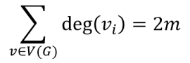
Theorem 2.1 handshaking lemma: given a graph G with a size of m, the sum of the degrees of the vertices is equal to 2m (or twice the total number of edges).

Eq.3

Theorem 2.2: every graph has and even number of odd vertices.
Theorem 2.3: given a graph G of order n and the relation below (in which u and v represent nonadjacent vertices), G is connected and diam(G)≤2.

Eq.4

Theorem 2.4: given a graph G of order n and δ(G)≥(n-1)/2, the graph G is connected.
Theorem 2.5: given integers r and n such that 0≤r≤n-1, there exists an r-regular graph of order n if and only if either r or n is even.
Theorem 2.6: for every graph H and every integer r≥Δ(G), there exists an r-regular graph G which contains H as an induced subgraph.
Theorem 2.7: a non-increasing sequence of nonnegative integers s~1~, s~2~, … s~n~ (where s~1~≥1) is graphical if and only if the sequence below is graphical.

Eq.5

Theorem 2.8: if a graph’s adjacency matrix A=a~ij~ is raised to a power k, then the entry a~ij~^k^ in row i and column j of A^k^ is equal to the number of distinct v~i~-v~j~ walks of length k within the graph.
Theorem 2.9 the party theorem: for any nontrivial simple graph, there exists a pair of vertices with the same degree. As such, no nontrivial simple graph is irregular.
Theorem 2.10: given a graph F with order k≥2 and a graph G which contains m copies of F as subgraphs, the equality below (involving the F-degree) is true.

Eq.6

Theorem 2.11: given a subgraph F with an even order and a graph G, the graph G has an even number of vertices with an odd F-degree.
Theorem 2.12: given a nontrivial connected graph F, there exists an F-irregular graph if and only if Fdeg≠2.
Theorem 2.13: given a connected graph G with an order of two or more, G is the underlying graph of an irregular multigraph or irregular weighted graph.
Theorem 2.14 Euler’s formula: given a graph with V vertices, E edges, and F faces (recall that the space outside of a graph is counted as a face) that is drawn without edge intersections, the relation below is always true.

Eq.7

Theorem 2.15: given an adjacency matrix A of a digraph D, the transposed matrix A^T^ is the adjacency matrix of a digraph R such that R is the graph transpose of D.

Theorems [3]

Theorem 3.1: two graphs are isomorphic if and only if their complements are isomorphic.
Theorem 3.2: two isomorphic graphs G and H possess identical sets of vertex degrees.
Theorem 3.3: two isomorphic graphs G and H possess the same structural properties. For instance, G is bipartite if and only if H is bipartite, G is connected if and only if H is connected, G contains a 3-cycle if and only if H contains a 3-cycle, etc.
Theorem 3.4: isomorphism is an equivalence relation on the set of all graphs and so isomorphism is reflexive (every graph is isomorphic to itself), symmetric (there exists an inverse for every isomorphism), and transitive (if G~1~≌G~2~ and G~2~≌G~3~, then G~1~≌G~3~).
Theorem 3.5: an edge e∈G is a bridge if and only if e does not lie on any cycles of G.
Theorem 3.6: a graph G is a tree if and only if every pair of vertices in G are connected by a unique path.
Theorem 3.7: every nontrivial tree has at least two end-vertices.
Theorem 3.8: every tree of order n has a size of n–1.
Theorem 3.9: every forest of order n with k components has a size of n–k.
Theorem 3.10: given a graph G of order n and size, if G satisfies any two of the following properties, then G is a tree. (i) G is connected, (ii) G is acyclic, (iii) m=n–1.
Theorem 3.11: if T is a tree with order k and G is a graph with minimum degree δ(G)≥k–1, then T is isomorphic to some subgraph of G.
Theorem 3.12: every connected graph contains at least one spanning tree.

Theorems [4]

Theorem 4.1: given a vertex v incident with a bridge within a connected graph G, v is a cut-vertex of G if and only if deg(v)≥2.
Theorem 4.2: given a connected graph G with an order of three or greater, if G contains a bridge, then G contains a cut-vertex.
Theorem 4.3: given a cut-vertex v in a connected graph G as well as vertices u and w that belong to distinct components of the disconnected graph G – v, the vertex v lies on every u-w path of G.
Theorem 4.4: a vertex v of a connected graph G is a cut-vertex if and only if there exist vertices u and w (distinct from v) such that v lies on every u-w path of G.
Theorem 4.5: consider a nontrivial connected graph G and vertices u,v∈V(G). If v is the farthest possible vertex from u as measured by d(u,v), then v is not a cut-vertex of G.
Theorem 4.6: every nontrivial connected graph contains at least two vertices which are not cut-vertices.
Theorem 4.7: given a graph G with an order of three or greater, G is nonseparable if and only if every two vertices lie on a common cycle.
Theorem 4.8: an equivalence relation R can be defined on the edge set of a nontrivial connected graph G for edges e,f∈E(G) when e=f or e and f lie on a common cycle of G.
Theorem 4.9: every two distinct blocks B~1~ and B~2~ in a nontrivial connected graph have the following properties. (i) B~1~ and B~2~ are edge disjoint, (ii) B~1~ and B~2~ have at most one common vertex, and (iii) if B~1~ and B~2~ share a common vertex v, then v is a cut-vertex of G.
Theorem 4.10: for every positive integer n, there exists a k-edge-connected graph K~n~ such that λ(K~n~)=n-1.
Theorem 4.11: for every graph G, the relation κ(G)≤λ(G)≤δ(G) holds. (Recall that δ(G) denotes a graph’s minimum degree).
Theorem 4.12: for a cubic graph (3-regular), then κ(G)=λ(G).
Theorem 4.13: if a graph has order n and size m≥n-1, then κ(G)≤2m/n.

Fig.7

Theorem 4.14 Menger’s theorem: given nonadjacent vertices u and v in a graph G, the minimum number of vertices in a u-v separating set equals the maximum number of internally disjoint u-v paths in G.
Theorem 4.15: a nontrivial graph G is k-connected for an integer k≥2 if and only if every pair of distinct vertices u,v∈G corresponds to at least k internally disjoint u-v paths in G.
Theorem 4.16: given a k-connected graph G any set S of k vertices in G, if a new vertex w is created and joined to the vertices of S, then the resulting graph is also k-connected.
Theorem 4.17: given a k-connected graph G and vertices k+1 distinct vertices of u,v~1~,v~2~,…,v~k~∈G; there exist internally disjoint u-v~i~ paths such that 1≤i≤k.
Theorem 4.18: given a k-connected graph G with k≥2, every k vertices of G lie on a common cycle of G.
Theorem 4.19: given distinct vertices u and v in a graph G, the minimum number of edges in G which separate u and v equals the maximum number of edge-disjoint u-v paths in G for each pair of distinct vertices u,v∈]
Theorem 4.20: a nontrivial graph G is k-edge-connected if and only if G contains k edge-disjoint u-v paths for each pair of distinct vertices u,v∈G.

Theorems [5]

Theorem 5.1: a connected graph G contains an Eulerian trail if and only if every vertex of G has an even degree or exactly two vertices of G have odd degrees. In the case of a graph with exactly two vertices of odd degree, each Eulerian trail begins at one of the vertices with an odd degree and ends at the other vertex with an odd degree.
Theorem 5.2: the Petersen graph is non-Hamiltonian.
Theorem 5.3: given a Hamiltonian graph G, then every nonempty proper subset S of vertices in G satisfies the relation k(G – S)≤|S|, where k(G – S) is the number of components in the graph G – S and |S| is the cardinality of S.
Theorem 5.4: if a graph G contains a cut-vertex, then G is not Hamiltonian.
Theorem 5.5: given a graph G with an order n≥3, if deg(u)+deg(v)≥n for every pair of nonadjacent vertices u,v∈G, then G is Hamiltonian.
Theorem 5.6: given a graph G with an order n≥3 and deg(v)≥n/2 for every vertex v∈G, then G is Hamiltonian.
Theorem 5.7: given two nonadjacent vertices u and v in a graph G of order n such that deg(u)+deg(v)n, G+uv is Hamiltonian if and only if G is Hamiltonian. Note that G+uv denotes the graph G with a new edge between vertices u and v (which were formerly nonadjacent).
Theorem 5.8: given a graph G with an order n≥3, if the relation 1≤j≤n/2 holds for every integer j and the number of vertices in G with a degree of at most j is less than j, then G is Hamiltonian.
Theorem 5.9 Handshaking lemma for digraphs: given a digraph D with size m and V(D)={v~1~,v~2~,…,v~n~}, the equation below holds.

Eq.12

Theorem 5.10: if a digraph D contains a u-v walk with a length of L, then D contains a u-v path with a length of at most L.
Theorem 5.11: a digraph D is strong if and only if D contains a closed spanning walk.
Theorem 5.12: a nontrivial connected digraph D is Eulerian if and only if od(v)=id(v) for each vertex v∈D.
Theorem 5.13: a nontrivial connected graph G has a strong orientation if and only if G does not contain any bridges.
Theorem 5.14: a tournament T is transitive if and only if T does not contain any cycles.
Theorem 5.15: if u is a vertex with a maximum outdegree for a tournament T, then d(u,v)≤2 for every vertex v∈T.
Theorem 5.16: every tournament T contains a Hamiltonian path.
Theorem 5.17: every vertex in a tournament T which is nontrivial and strongly connected belongs to a directed 3-cycle.
Theorem 5.18: a nontrivial tournament T is Hamiltonian if and only if T is strongly connected.
Theorem 5.19: given a strongly connected tournament T with an order n≥4, there exists a vertex v such that T – v is also a strongly connected tournament.

Application: methods of proof

[New mathematical concepts and tools are made through proofs. Using a series of logical steps, previously unrealized insights about the universe can be uncovered. Existing definitions and theorems are built upon, allowing an ever-expanding system of truth to develop, a system known as mathematics.

Direct proof: a sequence of statements which starts with a given statement p and ends by proving a statement q. Each successive statement must logically follow from the previous statement.
Proof by contradiction: by assuming that the negation of a statement q is true and then finding a logical contradiction, q can be proven. Negation is a logical operator denoted as ¬ If ¬q is true, then q is false. If ¬q is false, then q is true.
Contrapositive proof: the statements p⇒q and ¬p⇒¬q are logically equivalent, so p⇒q can be proven by proving the contrapositive ¬p⇒¬q.
Proving a biconditional: a logical biconditional is denoted as p⇔q, “p if and only if q,” p⇒q and q⇒p, or “p is necessary and sufficient for q.” Biconditionals can be proven in several ways. (i) By proving p⇒q and q⇒ (ii) By proving p⇒q and ¬p⇒¬q. (iii) By proving ¬q⇒¬p and q⇒p. (iv) By proving ¬q⇒¬p and ¬p⇒¬q.
Proof by induction: consider a true basis statement p~1~ that is true and an infinite sequence of statements p~1~⇒p~2~⇒p~3~⇒…⇒p~n~ such that each statement logically implies the next in the sequence. If we know that p~1~ is true, then all the other statements are also true. To prove by induction, show that p~1~ is true and then show that p~n~⇒p~n+1~ for all n.
Proof by cases: some proofs can be simplified by breaking the problem into cases and proving each case separately (i.e. proving a statement for even numbers and then for odd numbers).

Application: statistical properties of graphs

[Graph theoretic models of complex networks can be analyzed using statistical properties. Such properties are useful for many real-world technological, social, and biological networks. In particular, network properties have revealed insights about the brain and may serve as a quantitative diagnosis method for mental illnesses, neurodegenerative diseases, and other disorders of the nervous system.

Mean vertex degree: the average degree of vertices in a network.
Degree distribution: the set of all vertex degrees in a network ordered in a sequential manner (often by increasing degree value). Depending on the particular network, this can result in Gaussian, bimodal, skewed, or other types of distribution.
Assortativity: a measure of degree correlation between adjacent vertices, often described by an assortativity coefficient r, a Pearson correlation coefficient computed using the degrees of all adjacent vertex pairs in a network. In the formula below (for undirected networks), q~j~ represents the number of edges incident on a vertex j with the exception of the edge between vertex j and vertex k. Likewise, q~k~ represents the number of edges incident with a vertex k with the exception of the edge between vertex k and vertex j.

Eq.8

Clustering coefficient: given a vertex v, its clustering coefficient C is defined as the number of edges s among the set of N vertices adjacent to v over the maximum possible number of edges among said vertices. Note that this measure excludes the edges incident with v itself.]

Eq.9

Mean path length: the average number of vertices traversed by the paths in a network.
Efficiency: the inverse of a path length L given by 1/L, often used because it is more convenient for certain topological analyses of networks.
Connection density: given a network of order n, its connection density d (also called cost) is defined as the network’s size S over the size of a complete graph of order n.

Eq.10

Closeness centrality: a measure of how many shortest paths between all pairs of vertices in a network pass through a given vertex u. The higher the closeness centrality, the closer u is to all other vertices in the network. In the equation below, N is the network’s order and v represents all of the vertices such that v≠u.

Eq.11

Robustness: describes how much a network’s overall structure and statistical properties are altered upon perturbations like vertex deletions, edge deletions, vertex insertions, edge insertions, reversals of edge directionalities, and changes to edge weight. Robustness can be quantified by a diverse array of methods.
Modularity: a term describing networks which include densely interconnected subgraphs known as modules. Not many edges are formed between vertices within a given module and vertices outside of said module. Modularity can be quantified by a diverse array of methods.
Hubs: vertices with high closeness centrality values are called hubs. Alternatively, vertices with high degree can be called hubs.
Provincial hubs: vertices found inside of modules are often called provincial hubs.
Connector hubs: vertices which link distinct modules are often called connector hubs.
Small-worldness: a property proportional to a network’s mean clustering coefficient over its mean path length. Networks with high small-worldness are called small-world networks.

Eq.13

Scale-free: a network with a degree distribution that is described by a power law is a called scale-free. Power law distributions are defined by the probability mass function P(X=k)=k^-λ^ where k is the degree of a given vertex in the network and λ is a constant parameter specific to the network under investigation.

Application: the graph Laplacian and random walks

[The graph Laplacian (also called the Laplacian matrix) allows a variety of useful analyses to be carried out on graphs. In particular, it can probabilistically describe a random walker’s activities. Random walkers can be thought of as objects which stochastically “jump from vertex to vertex” on a graph.

Degree matrix: a matrix D with the degrees of a graph G along the diagonal. The remaining entries of D are zeros. For digraphs, the degree matrix may describe either the indegree or the outdegree.
Laplacian matrix: given a degree matrix D and an adjacency matrix A which describe some graph, the graph’s Laplacian matrix or graph Laplacian is L=D–A.
Random walk normalized Laplacian: a matrix defined by L^rw^=D^-1^ The random walk normalized Laplacian can also be computed by L^rw^=I~n~–D^-1^A where I~n~ is the identity matrix.
Transition matrix for a random walker: the term D^-1^A from the random walk normalized Laplacian represents the transition matrix P for a random walker on a graph G. For a vertex i∈G and the i^th^ standard basis vector e~i~, the vector x=e~i~P is a probability vector describing the distribution of a random walker’s possible locations after taking a single step from vertex i. (Note that a probability vector is a vector of values which sum to one and represent probabilities). If q~0~ is a probability vector describing the initial distribution of a random walker’s possible locations and q~t~ is a probability vector describing the distribution of the random walker’s possible locations after t steps, then q~t~=q~0~P^t^.

References

[Chartrand G, Zhang P. 2013. A First Course in Graph Theory. Dover Publications.
[Bullmore E, Sporns O. 2009. Complex brain networks: graph theoretical analysis of structural and functional systems. Nat Rev Neurosci 10:186.

Stop Thinking, Just Do!