Article Source

Title: Graph Embeddings — The Summary

Graph Embeddings — The Summary

This article presents what graph embeddings are, their use, and the comparison of the most commonly used graph embedding approaches.

Graphs are commonly used in different real-world applications. Social networks are large graphs of people that follow each other, biologists use graphs of protein interactions, while communication networks are graphs themselves. They use graphs of word co-occurrences in the field of text mining. The interest in performing machine learning on graphs is growing. They try to predict new friendships in social media, while biologists predict the protein’s functional labels. Mathematical and statistical operations on the graphs are limited and applying machine learning methods directly to graphs is challenging. In this situation, embeddings appear as a reasonable solution.

What are graph embeddings?

Graph embeddings are the transformation of graphs to a vector or a set of vectors. Embedding should capture the graph topology, vertex-to-vertex relationship, and other relevant information about graphs, subgraphs, and vertices. More properties embedder encode better results can be retrieved in later tasks. We can roughly divide embeddings into two groups:

Vertex embeddings: We encode each vertex (node) with its own vector representation. We would use this embedding when we want to perform visualization or prediction on the vertex level, e.g. visualization of vertices in the 2D plane, or prediction of new connections based on vertex similarities.
Graph embeddings: Here we represent the whole graph with a single vector. Those embeddings are used when we want to make predictions on the graph level and when we want to compare or visualize the whole graphs, e.g. comparison of chemical structures.

Later, we will present a few commonly used approaches from the first group (DeepWalk, node2vec, SDNE) and approach graph2vec from the second group.

Why we use graph embeddings?

Graphs are a meaningful and understandable representation of data, but there are a few reasons why graph embeddings are needed:

Machine learning on graphs is limited. Graphs consist of edges and nodes. Those network relationships can only use a specific subset of mathematics, statistics, and machine learning, while vector spaces have a richer toolset of approaches.
Embeddings are compressed representations. Adjacency matrix describes connections between nodes in the graph. It is a |V| x |V| matrix, where |V| is a number of nodes in the graph. Each column and each row in the matrix present a node. Non-zero values in the matrix indicate that two nodes are connected. Using an adjacency matrix as a feature space for large graphs is almost impossible. Imagine a graph with 1M nodes and an adjacency matrix of 1M x 1M. Embeddings are more practical than the adjacency matrix since they pack node properties in a vector with a smaller dimension.
Vector operations are simpler and faster than comparable operations on graphs.

Challenges

The embedding approach needs to satisfy more requirements. Here we describe three of many challenges for embedding methods:

We need to make sure that embeddings well describe the properties of the graphs. They need to represent the graph topology, node connections, and node neighborhood. The performance of prediction or visualization depends on the quality of embeddings.
The size of the network should not decrease the speed of the embedding process. Graphs are usually large. Imagine the social networks with millions of people. A good embedding approach needs to be efficient on large graphs.
An essential challenge is a decision on the embedding dimensionality. Longer embeddings preserve more information while they induce higher time and space complexity than sorter embeddings. Users need to make a trade-off based on the requirements. In articles, they usually report that embedding size between 128 and 256 are sufficient for most of the tasks. In the method Word2vec, they selected the embedding length 300.

Word2vec

Before we present approaches for embedding graphs, I will talk about the Word2vec method and the skip-gram neural network. They are a basis for graph embedding methods. If you want to understand it better, I suggest checking this excellent tutorial or this video.

Word2vec is an embedding method which transforms words into embedding vectors. Similar words should have similar embeddings. Word2vec uses the skip-gram network which is the neural network with one hidden layer. The skip-gram is trained to predict neighbor word in the sentence. This task is named a fake task since it is just used in a training phase. Network accepts the word at the input and is optimized such that it predicts the neighbor words in a sentence with high probability. The figure below shows the example of input words (marked with green) and words which are predicted. With this task authors achieve that two similar words have similar embeddings since it is likely that two words with similar meaning have similar neighborhood words.

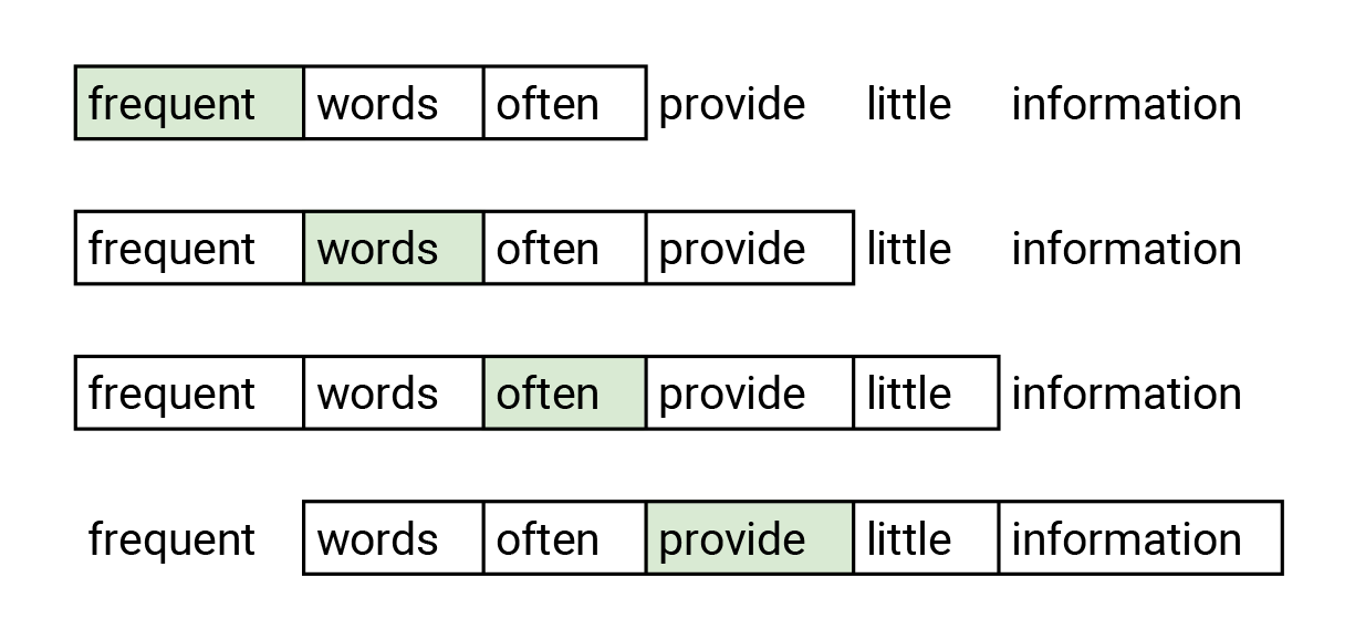
The word colored with green is given to the network. It is optimized to predict the word in the neighborhood with higher probability. In this example, we consider words that are the most two places away from the selected words. The skip-gram neural network seen in the figure below has the input layer, one hidden layer, and the output layer. The network accepts the one-hot encoded words. One-hot encoding is a vector with length same than the word dictionary and has all zeros except one. Number one is on the place where an encoded word appears in the dictionary. The hidden layer has no activation function, its output presents an embedding of the word. The output layer is a softmax classifier that predicts neighborhood words. More details about skip-gram are available in the tutorial I mentioned before .

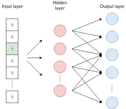
Skip-gram neural network

I will present four graph embedding approaches. Three of them embed nodes, while one embeds the whole graph with one vector. They use the embedding principle from Word2vec in three approaches.

Vertex embedding approaches

I will present three methods that embed nodes in the graph. They are selected since they commonly used in practice and usually provide the best results. Before we dive in, I may mention that approaches for node embedding can be divided into three major groups: factorization approaches, random walk approaches, and deep approaches.

DeepWalk uses random walks to produce embeddings. The random walk starts in a selected node then we move to the random neighbor from a current node for a defined number of steps.

The method basically consists of three steps:

Sampling: A graph is sampled with random walks. Few random walks from each node are performed. Authors show that it is sufficient to perform from 32 to 64 random walks from each node. They also show that good random walks have a length of about 40 steps.
Training skip-gram: Random walks are comparable to sentences in word2vec approach. The skip-gram network accepts a node from the random walk as a one-hot vector as an input and maximizes the probability for predicting neighbor nodes. It is typically trained to predict around 20 neighbor nodes — 10 nodes left and 10 nodes right.
Computing embeddings: Embedding is the output of a hidden layer of the network. The DeepWalk computes embedding for each node in the graph.

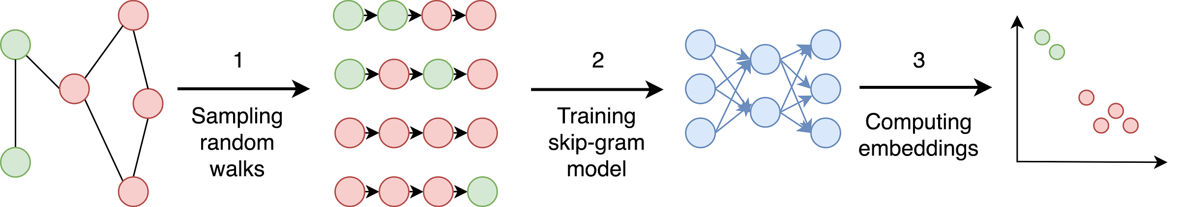
Phases of DeepWalk approach

DeepWalk method performs random walks randomly what means that embeddings do not preserve the local neighborhood of the node well. Node2vec approach fixes that.

Node2vec is a modification of DeepWalk with the small difference in random walks. It has parameters P and Q. Parameter Q defines how probable is that the random walk would discover the undiscovered part of the graph, while parameter P defines how probable is that the random walk would return to the previous node. The parameter P control discovery of the microscopic view around the node. The parameter Q controls the discovery of the larger neighborhood. It infers communities and complex dependencies.

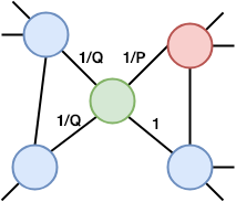
The figure shows probabilities of a random walk step in Node2vec. We just made a step from the red to the green node. The probability to go back to the red node is 1/P, while the probability to go the node not connected with the previous (red) node 1/Q. The probability to go to the red node’s neighbor is 1. Other steps of the embedding are the same than the DeepWalk approach.

Structural Deep Network Embedding (SDNE) does not have any in common with previous two approaches since it does not perform random walks. I mention it since it is very constant in its performance on different tasks.

It is designed so that embeddings preserve the first and the second order proximity. The first-order proximity is the local pairwise similarity between nodes linked by edges. It characterizes the local network structure. Two nodes in the network are similar if they are connected with the edge. When one paper cites other paper, it means that they address similar topics. The second-order proximity indicates the similarity of the nodes’ neighborhood structures. It captures the global network structure. If two nodes share many neighbors, they tend to be similar.

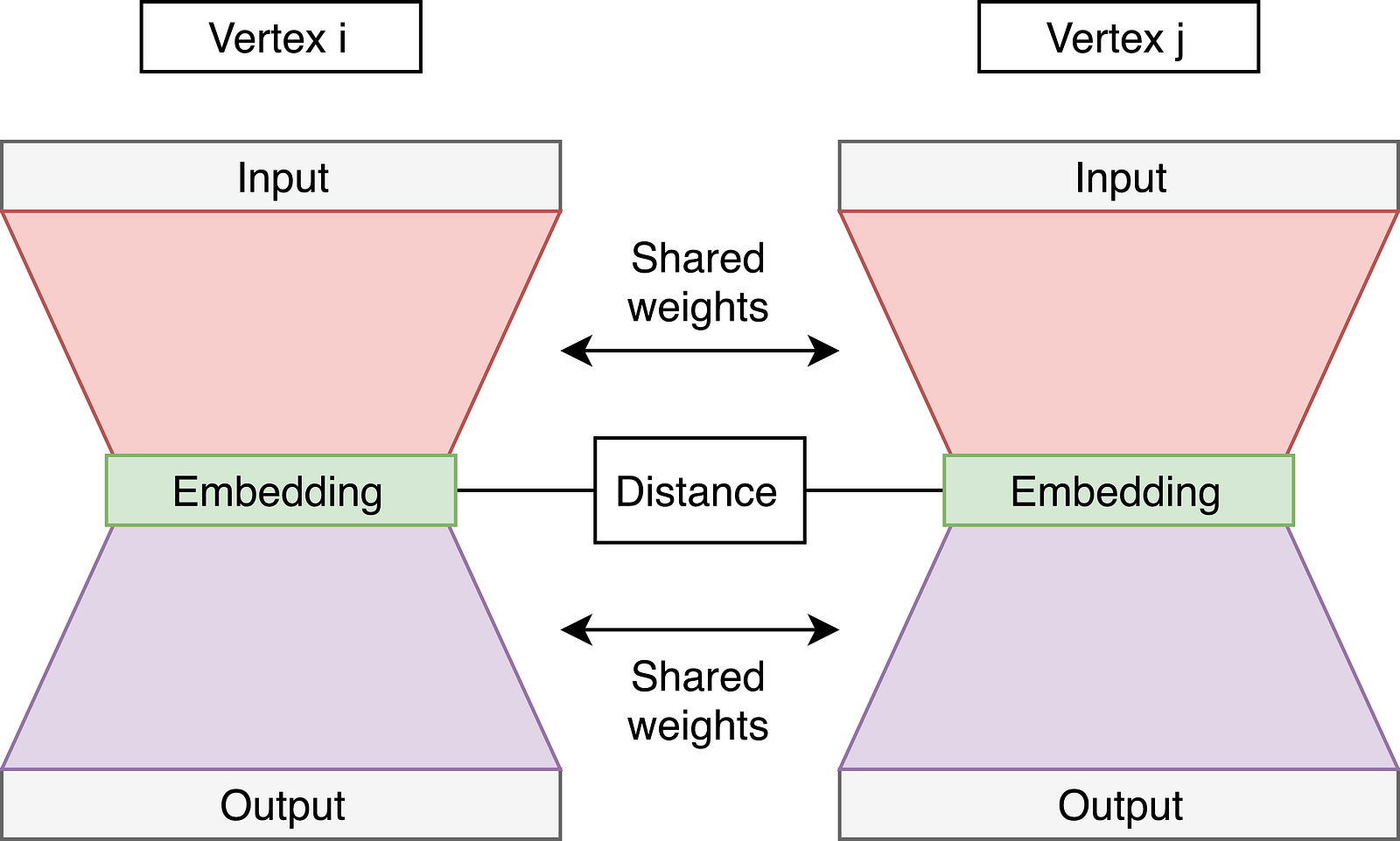
Authors present an autoencoder neural network which has two parts — see figure below. Autoencoders (left and right network) accept node adjacency vector and are trained to reconstruct node adjacency. These autoencoders are named vanilla autoencoders and they learn the second order proximity. Adjacency vector (a row from adjacency matrix) has positive values on places that indicate nodes connected to the selected node.

There is also a supervised part of the network — the link between the left and the right wing. It computes the distance between embedding from the left and the right part and includes it in the common loss of the network. The network is trained such that left and right autoencoder get all pairs of nodes which are connected by edges on the input. The loss of a distance part helps in preserving the first order proximity.

The total loss of the network is calculated as a sum of the losses from the left and the right autoencoder combined with the loss from the middle part.

Graph embedding approach

The last approach embeds the whole graph. It computes one vector which describes a graph. I selected the graph2vec approach since it is as I know the best performing approach for a graph embedding.

Graph2vec is based on the idea of the doc2vec approach that uses the skip-gram network. It gets an ID of the document on the input and is trained to maximize the probability of predicting random words from the document.

Graph2vec approaches consist of three steps:

Sampling and relabeling all sub-graphs from the graph. Sub-graph is a set of nodes that appear around the selected node. Nodes in sub-graph are not further than the selected number of edges away.
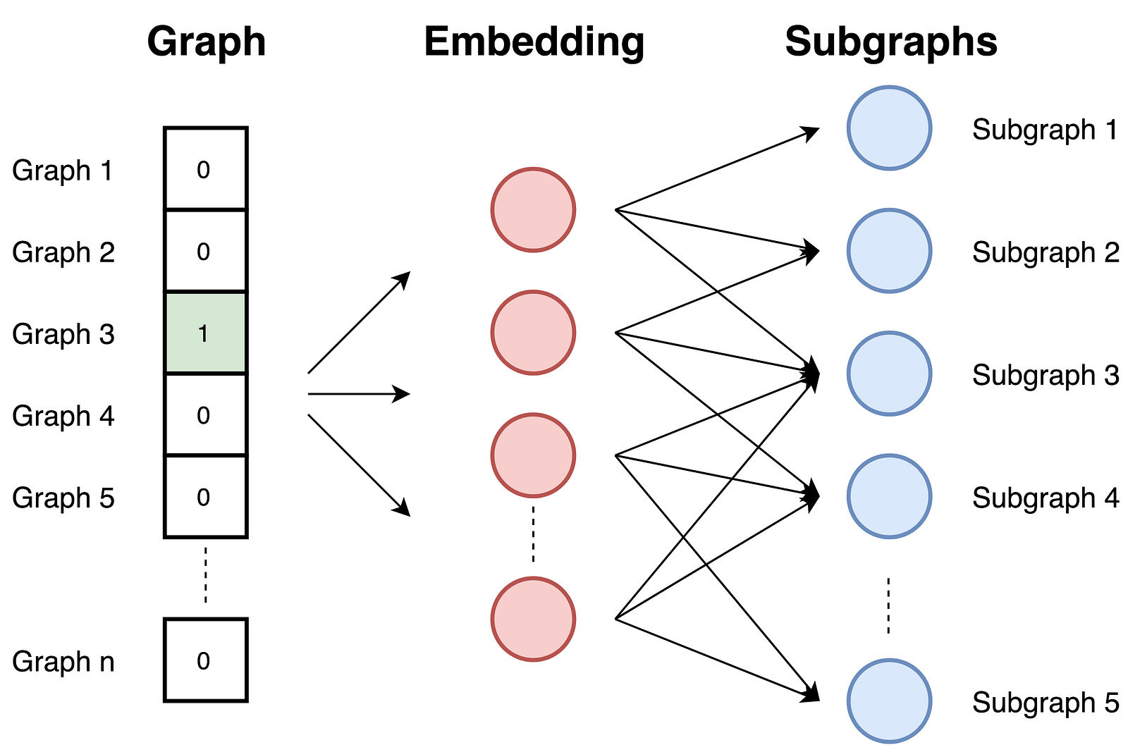
Training the skip-gram model. Graphs are similar to documents. Since documents are set of words graphs are set of sub-graphs. In this phase, the skip-gram model is trained. It is trained to maximize the probability of predicting sub-graph that exists in the graph on the input. The input graph is provided as a one-hot vector.
Computing embeddings with providing a graph ID as a one-hot vector at the input. Embedding is the result of the hidden layer.

Since the task is predicting sub-graphs, graphs with similar sub-graphs and similar structure have similar embeddings.

Other embedding approaches

I presented four approaches that are based on the literature frequently used. Since this topic is currently very popular, more approaches are available. Here I present a list of other available approaches:

Vertex embedding approaches: LLE, Laplacian Eigenmaps, Graph Factorization, GraRep, HOPE, DNGR, GCN, LINE
Graph embedding approaches: Patchy-san, sub2vec (embed subgraphs), WL kernel andDeep WL kernels

References

[1] C. Manning, R. Socher, Lecture 2 | Word Vector Representations: word2vec (2017), YouTube.

[2] B. Perozzi, R. Al-Rfou, S. Skiena, DeepWalk: Online Learning of Social Representations (2014), arXiv:1403.6652.

[3] C. McCormick. Word2Vec Tutorial — The Skip-Gram Model(2016), http://mccormickml.com.

[4] T. Mikolov, K. Chen, G. Corrado, J. Dean, Efficient Estimation of Word Representations in Vector Space (2013), arXiv:1301.3781.

[5] A. Narayanan, M. Chandramohan, R. Venkatesan, L. Chen, Y. Liu, S. Jaiswal, graph2vec: Learning Distributed Representations of Graphs (2017), [*arXiv:1707.05005](https://arxiv.org/abs/1707.05005).*

[6] P. Goyal, E. Ferrara, Graph Embedding Techniques, Applications, and Performance: A Survey (2018), Knowledge-Based Systems.

[7] D. Wang, P. Cui, W. Zhu, Structural Deep Network Embedding (2016), Proceedings of the 22nd ACM SIGKDD international conference on Knowledge discovery and data mining.

[8] A. Grover, J. Leskovec, node2vec: Scalable Feature Learning for Networks (2016), Proceedings of the 22nd ACM SIGKDD international conference on Knowledge discovery and data mining.

Stop Thinking, Just Do!