Article Source

• Title: Transfer Learning — part 1

---

Transfer Learning — Part I

Introduction

What is transfer learning (TL) and how it is different from classical machine learning (ML)?

The big lie of ML is that the distribution of the training data is the same as the distribution of the data on which the model is going to be used. What if this assumption is violated that is the data has different distribution over different feature space?

When enough data are available, one can simply retrain a model on the new data and discard old data altogether. This is not always possible. However, there is a way to improve. If it is known that there is a relationship between training data and other data, the transfer of knowledge (or transfer learning) obtained on training data to a model for other data can help.

Transfer learning is different from classical ML setup: instead of learning in one setting, the knowledge from learning in one setting is reused to improve learning in another setting. Transfer learning is inspired by the way human learners take advantage of their existing knowledge and skills: a human who knows how to read literature is more likely to succeed in reading scientific papers than a human who does not know how to read at all. In the context of supervised learning, transfer learning implies the ability to reuse the knowledge of the dependence structure between features and labels learned in one setting to improve the inference of the dependence structure in another setting. At Dataswati, we are particularly interested in this type of transfer learning applied to time-series data from different factories and I have personally spent a fair share of my time working on these problems.

In this post, I will review different aspects of transfer learning, but first, a couple of words about classical supervised machine learning setting.

Supervised machine learning: a quick recap

We have a dataset D that contains samples of feature vectors (x ∈ 𝒳) and corresponding labels (y ∈ 𝒴): D = {(xi, yi) : i = 1,…,m}. D consists of the set of training examples D|X = {xi : i = 1,…,m}, and the set of corresponding labels D|Y = {yi : i = 1,…,m}. Here m is sample size. All pairs (x, y) are assumed to be independently sampled form the same joint-distribution P(X, Y) (i.i.d. assumption) that reflects the dependence between random variables X and Y. In other words, (xi, yi) is a realization of (X, Y) ∼ P(X, Y) for all i. Our goal is to use D to learn a function h : 𝒳 → 𝒴 (h for “hypothesis”) so that h approximates true relationship between x and y, that is some summary of P(Y|X = x), for example h(x) ≈ E(Y|X = x). When we are searching for a good h, we constrain our search to some class of functions ℋ (e.g. class of linear models), h ∈ ℋ. If ℋ is not too complex and sample size m is large enough, we can learn “good” h (e.g. using Empirical Risk Minimization :

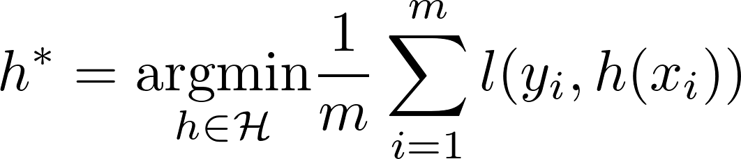
ERM algorithm , where l is some loss function) so that h provides a good approximation of the true relationship between x and y not only on (x, y) ∈ D, but on the other data (x, y) sampled from P(X, Y).

What if we don’t have enough data or we don’t have labels? Is there a hope?

What if…

• …we have several different datasets, but with similar X-Y dependence structure?
• …we have labels only for some of these datasets, but not the others and we want to make predictions when no labels are available?
• …we want to learn dependence on a dataset with small sample size when we have another dataset with large sample size and similar, but different dependence structure?
• …we have a combination of all of these?

Indeed, there is a hope, and it is called…

 …transfer learning.

Pan, Yang, and others (2010) and Weiss, Khoshgoftaar, and Wang (2016) give a great overview of transfer learning prior to Deep Learning craze. Pan, Yang, and others (2010) defines domain 𝒟 as a feature space considered together with the probability distribution over this space 𝒟 = (𝒳, P(X)). A task is formally defined as 𝒯 = (𝒴, f), here f is true, but unknown (and possibly stochastic) function f : 𝒳 → 𝒴 that we are trying to approximate with h ∈ ℋ.

To define the basic types of transfer learning (TL), let’s consider a simplified set up when we have just two domains with one task per domain: source domain 𝒟S and task 𝒯S, and target domain 𝒟T and task 𝒯T. In this simple setting, TL aims to improve learning of fT by using knowledge in 𝒯S, 𝒟S in addition to 𝒯T, 𝒟T, when 𝒯S ≠ 𝒯T or 𝒟S ≠ 𝒟T.

The table below summarizes types of TL compared to classical ML.

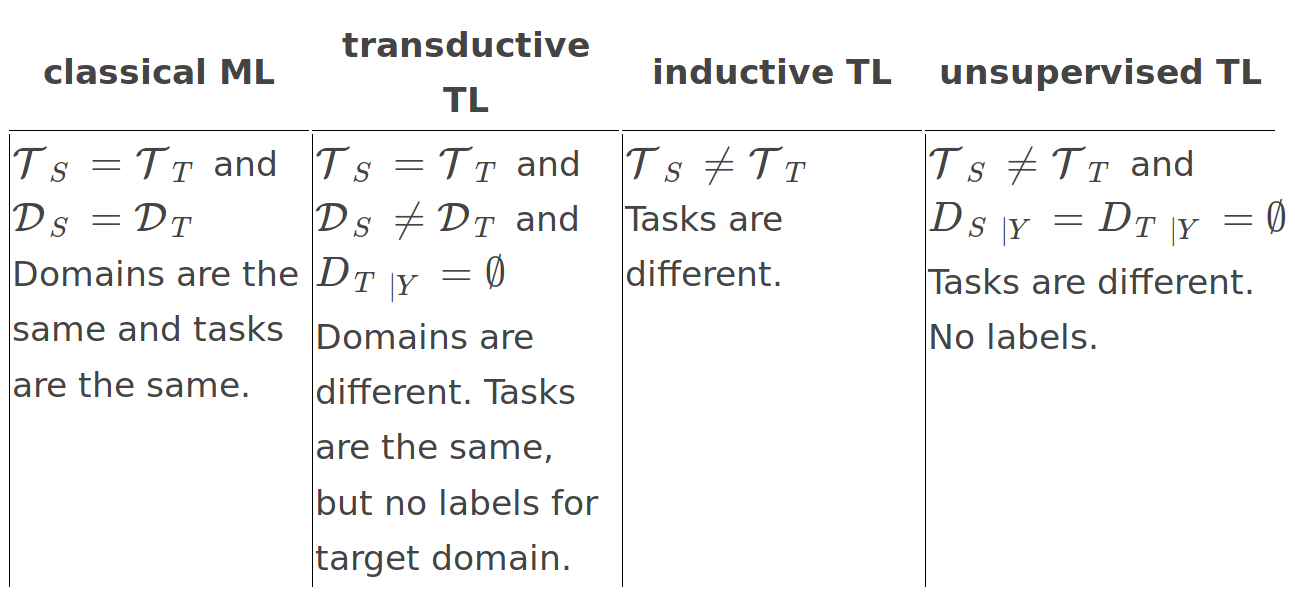
Types of transfer learning: inductive, transductive, and unsupervised Additional classification can be done based on feature spaces:

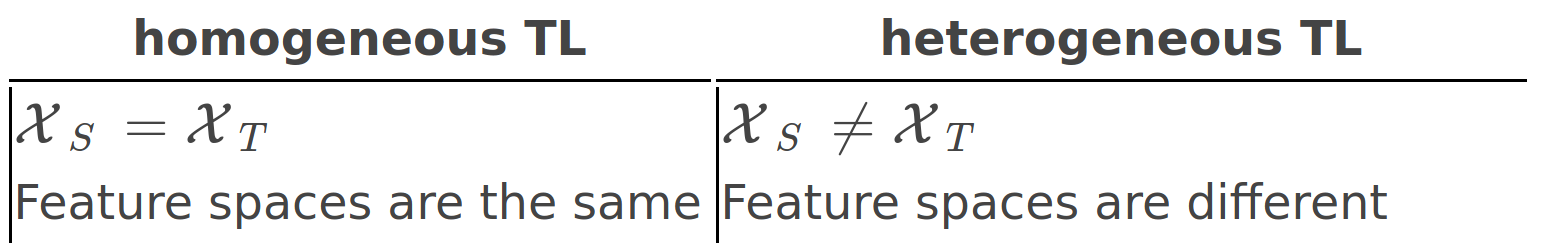
Homogeneous and heterogeneous transfer learning The most general case of transfer learning is when both feature spaces and distributions are different as well as tasks are different.

Pan, Yang, and others (2010) groups the approaches to TL based on “What to transfer” question:

• Instance-based transfer learning. It is assumed that some data from source domain can be reused in target domain. Importance sampling and instance reweighting are used here.
• Feature-representation transfer. A feature representation r is learned to facilitate modeling the dependence between r(X) and Y. It is then used to improve performance on target task. In the context of neural networks, one can train a supervised model in source domain and then take representation from one of the last layers to transform the data in target domain and then train another model on this transformed data.
• Parameter transfer. Source and target tasks are assumed to share some parameters or priors. In a simple case when hS, hT ∈ ℋ, hS = f(x; θS), hT = f(x; θT), it means that θS is partially similar to θT. In the context of neural networks, one can take a pretrained model like VGG and retrain last layers on one’s own task-specific data (retraining a small part of θS).

Recent TL developments relevant to Dataswati problems

In these series of posts, I will review some recent developments in TL including domain adaptation, few-shot learning, and the most general setting of multi-domain transfer learning.

Domain adaptation

In the framework of homogeneous transductive TL (𝒳S = 𝒳T = 𝒳), domain adaptation (training a model on the data from one joint-distribution and using it on the data from another one) has received substantial attention in the last decade, particularly, in the context of Deep Learning.

One often wants to find transformations ϕS, ϕT : 𝒳 → 𝒳̃ so that the distribution of transformed target data is the same as the distribution of transformed source data, that is P(ϕS(X)) = P(ϕT(X)) for X ∈ 𝒳, or particular case, when the transformation is only applied to source data: ϕS(X) ∼ P(X). The hope here is that we can efficiently apply the model trained on transformed source data to transformed target data.

Domain adaptation was theoretically investigated in the context of classification (Ben-David et al. 2007, 2010) and regression (Cortes and Mohri 2011) problems. Ben-David et al. (2007) studied the conditions under which a classifier trained on source domain data can be used in the target domain. They proved the upper bound on the error in target domain that was expressed as a function of the error in source domain. They further extended their analysis in Ben-David et al. (2010). In summary, the theory suggests that for an effective domain adaptation, one needs to train a model on a data representation from which it is impossible to discriminate between the source and the target domains.

I first mention some general approaches.

General approaches

A very simple approach to domain adaptation was proposed by Daumé III (2009). Daumé III (2009) transformed domain adaptation problem to a supervised learning problem by applying a simple data augmentation (duplicating features or filling with zeros) to both source and target domain and then training a model on augmented data pulled together from both domains. Their approach however requires labeled data in target domain (DT ∣ Y ≠ ∅).

Without labeled data in target domain, one can find transformations that align source and target distributions. Sun, Feng, and Saenko (2016) proposed CORrelation ALignment (CORAL) algorithm that aligns the second-order statistics of source and target distributions. Sun, Feng, and Saenko (2016) showed that CORAL can outperform some modern Deep Learning based approaches.

Si, Tao, and Geng (2010) used Bregman divergence -based regularization for cross-domain unsupervised dimensionality reduction and proposed transfer learning-aware versions of PCA, Fisher’s linear discriminant analysis (FLDA), locality preserving projections (LPP), marginal Fisher’s analysis (MFA), and discriminative locality alignment (DLA). Bregman divergence was used to minimize the difference between the distributions of projected data in source and target domains.

In their Transfer Component Analysis (TCA), Pan et al. (2011) used Maximum Mean Discrepancy (MMD) as a measure of distribution distance. MMD was used to learn the transformation (transfer components) of the dataset so that distribution distance was minimized. Long et al. (2013) proposed joint distribution adaptation (JDA) that generalizes TCA by including the objective of the minimization of conditional distribution.

Recently, Optimal Transport was successfully used for domain adaptation (Courty, Flamary, and Tuia 2014; Courty, Flamary, Tuia, et al. 2017; Courty, Flamary, Habrard, et al. 2017). Optimal Transport finds a transformation of the data in one domain to another domain by minimizing Wasserstein distance between distributions (Peyré, Cuturi, and others 2017).

In the context of mixture model-based learning, Beninel et al. (2012) proposed a method of mapping source data so that the distribution that models transformed data is equal to the distribution that models the target.

Deep Learning

Glorot, Bordes, and Bengio (2011) used feature representation based domain adaptation in the context of sentiment classification. Using reduced version of the Amazon dataset that included data in four different domains, they first pulled together data from all the domains and learned an unsupervised feature representation using Stacked Denoising Autoencoder (Vincent et al. 2008) on bag-of-words representation of the data. Then, for each source-target pair of domains, they trained binary SVM classifier on the representation of source data and used it on the representation of target data.

Ganin and Lempitsky (2014) proposed neural a network architecture that combined domain adaptation and deep feature learning within one training process. Similarly to adversarial training (Goodfellow et al. 2014), they simultaneously trained two models i) the domain classifier network to discriminate between transformed source and target data, and ii) predictor network that is trained to predict labels in source domain as well as to “fool” the domain classifier (achieved with a regularization term in its loss function). However, instead of alternating training of domain classifier and predictor, they introduced gradient reversal layer that allowed end-to-end training. They demonstrated efficiency of their approach on series of computer vision datasets: SVHN, MNIST, and traffic signs datasets. Ajakan et al. (2014) efficiently applied a very similar model to Amazon reviews sentiment analysis dataset. Ganin et al. (2016) presents extended analysis of such neural networks, so-called domain-adversarial adaptation neural networks.

References

Ajakan, Hana, Pascal Germain, Hugo Larochelle, François Laviolette, and Mario Marchand. 2014. “Domain-Adversarial Neural Networks.” arXiv Preprint arXiv:1412.4446.

Ben-David, Shai, John Blitzer, Koby Crammer, Alex Kulesza, Fernando Pereira, and Jennifer Wortman Vaughan. 2010. “A Theory of Learning from Different Domains.” Machine Learning 79 (1–2): 151–75.

Ben-David, Shai, John Blitzer, Koby Crammer, and Fernando Pereira. 2007. “Analysis of Representations for Domain Adaptation.” In Advances in Neural Information Processing Systems, 137–44.

Beninel, Farid, Christophe Biernacki, Charles Bouveyron, Julien Jacques, and Alexandre Lourme. 2012. Parametric Link Models for Knowledge Transfer in Statistical Learning. Nova Publishers.

Cortes, Corinna, and Mehryar Mohri. 2011. “Domain Adaptation in Regression.” In International Conference on Algorithmic Learning Theory, 308–23. Springer.

Courty, Nicolas, Rémi Flamary, Amaury Habrard, and Alain Rakotomamonjy.

1. “Joint Distribution Optimal Transportation for Domain Adaptation.” In Advances in Neural Information Processing Systems, 3730–9.

Courty, Nicolas, Rémi Flamary, and Devis Tuia. 2014. “Domain Adaptation with Regularized Optimal Transport.” In Joint European Conference on Machine Learning and Knowledge Discovery in Databases, 274–89. Springer.

Courty, Nicolas, Rémi Flamary, Devis Tuia, and Alain Rakotomamonjy.

1. “Optimal Transport for Domain Adaptation.” IEEE Transactions on Pattern Analysis and Machine Intelligence 39 (9): 1853–65.

Daumé III, Hal. 2009. “Frustratingly Easy Domain Adaptation.” arXiv Preprint arXiv:0907.1815.

Ganin, Yaroslav, and Victor Lempitsky. 2014. “Unsupervised Domain Adaptation by Backpropagation.” arXiv Preprint arXiv:1409.7495.

Ganin, Yaroslav, Evgeniya Ustinova, Hana Ajakan, Pascal Germain, Hugo Larochelle, François Laviolette, Mario Marchand, and Victor Lempitsky.

1. “Domain-Adversarial Training of Neural Networks.” The Journal of Machine Learning Research 17 (1): 2096–30.

Glorot, Xavier, Antoine Bordes, and Yoshua Bengio. 2011. “Domain Adaptation for Large-Scale Sentiment Classification: A Deep Learning Approach.” In Proceedings of the 28th International Conference on Machine Learning (ICML-11), 513–20.

Goodfellow, Ian, Jean Pouget-Abadie, Mehdi Mirza, Bing Xu, David Warde-Farley, Sherjil Ozair, Aaron Courville, and Yoshua Bengio. 2014. “Generative Adversarial Nets.” In Advances in Neural Information Processing Systems, 2672–80.

Long, Mingsheng, Jianmin Wang, Guiguang Ding, Jiaguang Sun, and Philip S Yu. 2013. “Transfer Feature Learning with Joint Distribution Adaptation.” In Proceedings of the IEEE International Conference on Computer Vision, 2200–2207.

Pan, Sinno Jialin, Ivor W Tsang, James T Kwok, and Qiang Yang. 2011. “Domain Adaptation via Transfer Component Analysis.” IEEE Transactions on Neural Networks 22 (2): 199–210.

Pan, Sinno Jialin, Qiang Yang, and others. 2010. “A Survey on Transfer Learning.” IEEE Transactions on Knowledge and Data Engineering 22 (10): 1345–59.

Peyré, Gabriel, Marco Cuturi, and others. 2017. “Computational Optimal Transport.”

Si, Si, Dacheng Tao, and Bo Geng. 2010. “Bregman Divergence-Based Regularization for Transfer Subspace Learning.” IEEE Transactions on Knowledge and Data Engineering 22: 929–42.

Sun, Baochen, Jiashi Feng, and Kate Saenko. 2016. “Return of Frustratingly Easy Domain Adaptation.” In AAAI, 6:8.

Vincent, Pascal, Hugo Larochelle, Yoshua Bengio, and Pierre-Antoine Manzagol. 2008. “Extracting and Composing Robust Features with Denoising Autoencoders.” In Proceedings of the 25th International Conference on Machine Learning, 1096–1103. ACM.

Weiss, Karl, Taghi M Khoshgoftaar, and DingDing Wang. 2016. “A Survey of Transfer Learning.” Journal of Big Data 3 (1): 9.