HIVE 0.14 Cost Based Optimizer (CBO) Technical Overview

CBO’s efficient execution plans, optimized techniques and performance gains

Analysts and data scientists⎯not to mention business executives⎯want Big Data not for the sake of the data itself, but for the ability to work with and learn from that data. As other users become more savvy, they also want more access. But too many inefficient queries can create a bottleneck in the system.

The good news is that Apache™ Hive 0.14—the standard SQL interface for processing, accessing and analyzing Apache Hadoop® data sets—is now powered by Apache Calcite. Calcite is an open source, enterprise-grade Cost-Based Logical Optimizer (CBO) and query execution framework.

The main goal of a CBO is to generate efficient execution plans by examining the tables and conditions specified in the query, ultimately cutting down on query execution time and reducing resource utilization. Calcite has an efficient plan pruner that can select the cheapest query plan. All SQL queries are converted by Hive to a physical operator tree, optimized and converted to Tez/MapReduce jobs, then executed on the Hadoop cluster. This conversion includes SQL parsing and transforming, as well as operator-tree optimization.

Query optimizers tend to have the biggest performance impact in a data warehouse system, since generating the right (or wrong) execution plan could mean the difference of seconds, minutes, or even hours in query execution time.

Performance testing of Hive 0.14 shows an average speedup of 2.5 times for TPC-DS benchmarked queries against a 30TB TPC-DS dataset. In our tests, total workload runtime shrank from 20.6 to 9 hours. In the current world of cloud computing, this improved performance directly translates into reduced operating costs.

In this post, we will dig into how this CBO works, including the background and challenges of query optimization, such as cardinality estimation and join ordering. We’ll also provide in-depth analysis of TPC-DS 30TB results.

The process of query optimization

Within a CBO, a query undergoes four distinct phases of examination and evaluation:

Parse and validate query The query is parsed, assuming the query is valid; the output of this phase is a logical tree (abstract syntax tree) that represents the operations that the query must perform, such as reading a particular table or performing an inner join.
Generate possible execution plans Using the logical tree created in step one, the CBO will produce other logically equivalent plans that can also get to the answers you’re looking for, by applying equivalence rules. The current model favors bushy plans (for reasons explained in more detail below) and is execution-engine agnostic.
For each logically equivalent plan, assign a cost The CBO will use number of distinct values-based heuristics to estimate selectivity and cardinality of each operator (to diminish the impact of inaccurate estimates during optimization) to calculate cost.
Select the plan with the lowest estimated cost

Query optimizer challenges

Two of the biggest difficulties to overcome in creating an efficient query are join optimization and table size when using table and column statistics. First, some definitions—then we’ll look at how Hive 0.14 CBO deals with these issues.

A join combines rows from two tables by using the values of fields common to each of them. The order used to join tables greatly influences the intermediary data set size, which impacts performance. The number of possible join orders increases exponentially with the number of tables involved. Coming up with all possible join orders is not practically feasible. Hence, one of the main benefits of the query optimizer is the ability to find the most efficient join order. The join order in the execution plan is not defined by the order of the tables in the query.

The query optimizer considers two different types of trees: left deepand bushy
Left deep: All internal nodes of a left-deep tree have at least one leaf as a child. This is simple to implement, but doesn’t produce efficient plans for snowflake schemas.

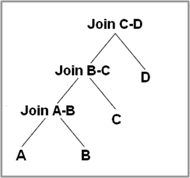
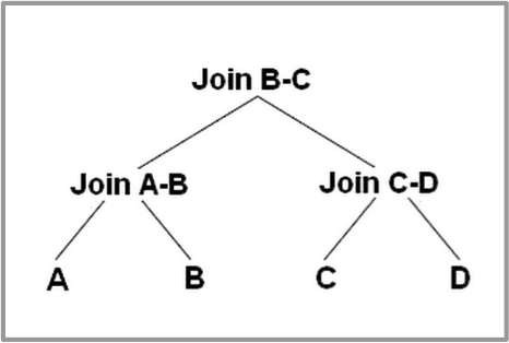
Bushy trees: When a join operates on two results of joins, as opposed to always having one table scan as input, you get a bushy tree. The join tree can take any shape. It is useful for snowflake schemas, as its search space is a lot bigger compared to left-deep trees. Bushy join trees also tend to contain subtrees that reduce intermediary data set size, and their joins with other subtrees tend to be more efficient than joins in the left-deep tree.

The CBO uses column and table statistics stored in the Hive metastore to create query plans that improve query performance. Statistics for the CBO are objects that contain information about the columns and partitions of a table. The CBO uses these statistics to estimate the cardinality and number of distinct values, etc. These estimates then help generate highly efficient query plans.

Currently, the CBO uses and maintains table cardinality and boundary statistics: min, max, avg, and number of distinct values. In the absence of histograms, cardinality can be assumed to follow uniform distribution.

Plans generated by the CBO are only as good as the quality of the statistics, so having up-to-date statistics is crucial. In Hive 0.14, the statistics creation DDL (data definition language) has been simplified and performance has vastly improved.

New CBO optimization in Hive 0.14

In Hive 0.14, we introduced new query optimization. Let’s take a look at these techniques and their impact on query optimization.

Join ordering optimization
Bushy join support
Join simplification

1. Join ordering optimization

Join ordering optimization plays a central role in the processing of relational database queries. Our goal is to find a join order with the lowest cost. The initial step is for the CBO to find the join order that results in the biggest reduction of intermediary rows as early as possible in the plan tree.

In Hive 0.14, the CBO uses boundary statistics to compute operator cardinality and join selectivity. Based on this information, the most efficient join order is selected.

To better understand the impact of join ordering, let’s look at TPC-DS Q3:

select 
    dt.d_year,
    item.i_brand_id brand_id,
    item.i_brand brand,
    sum(ss_ext_sales_price) sum_agg
from
    date_dim dt,
    store_sales,
    item
where
    dt.d_date_sk = store_sales.ss_sold_date_sk
        and store_sales.ss_item_sk = item.i_item_sk
        and item.i_manufact_id = 436
        and dt.d_moy = 12
group by dt.d_year , item.i_brand , item.i_brand_id
order by dt.d_year , sum_agg desc , brand_id
limit 10

The query above involves an equi-join between a fact table—store_sales (82B)—and two dimension tables, date_dim (73K) and item (462K). Each of the dimension tables has a filter, achieving the goal of reducing intermediary data as early as possible. The CBO should first join with the table that is most likely to reduce rows.

Graph 1: join graph for TPC-DS Q3

By analyzing min, max, number of distinct values (NDV) and row count for the join columns, the CBO is able to deduce that the joins involved are one-to-many joins⎯and that selectivity on the dimension table is likely to translate to a similar reduction of rows when joined with the fact table. Using that information, the CBO will order joins based on the estimated selectivity.

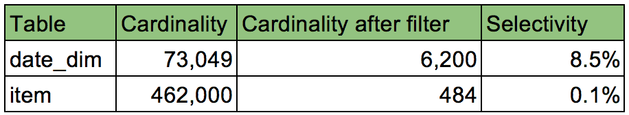
Table 1: dimension table cardinality and selectivity for TPC-DS Q3

Table 1 lists various statistics: the cardinality of each dimension table, the cardinality after applying filters, and selectivity, which is calculated by dividing the row count after filter by the row count before filter.

Join ordering optimization: results

The join trees in Graph 2 reflect the join tree generated by the Hive Explain Plan.

CBO ON

The CBO analyzes the join selectivity of item and date_dim. Using statistics, the CBO is able to deduce that joining store_sales with the item is more selective than joining store_sales with date_dim.

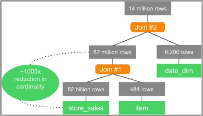
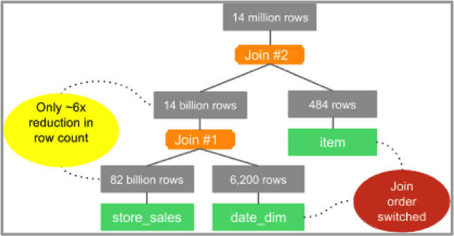
Graph 2: join tree for TPC-DS Q3 with CBO ON

As a result, the join reduces the number of rows coming out of store_sales from 82 billion to 82 million. Next, a join with date_dim follows this join, with the less selective join.

CBO OFF

When the CBO is turned off, the following join tree is produced:

Graph 3: join tree for TPC-DS Q3 with CBO OFF

In this case, the join order follows the order of tables in the query, and the join tree joins store_sales with date_dim first, which is the least selective join in the query. As a result, we end up with 14 billion rows of intermediary data without the CBO, compared to 82 million with the CBO enabled.

Join ordering optimization: interpreting the results

To understand the impact of the change in join order, the same query was run with CBO ON and then with CBO OFF. The results showed that the execution plan created by the CBO resulted in a 60% improvement in response time and CPU utilization.

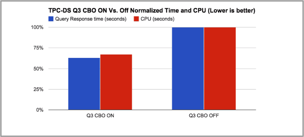
Graph 4: elapsed time and CPU for TPC-DS Q3 with CBO ON vs. OFF

Table 2 shows how optimal join ordering impacts query execution, in which CPU response time is cut by 50% and intermediary rows are reduced 161 times.

Table 2: elapsed time and CPU for TPC-DS Q3 with CBO ON vs. OFF

2. Bushy join support

Star and snowflake schemas are often found in data warehousing systems. These schemas are represented by centralized fact tables connected to multiple dimensions, splitting up data into dimension tables and avoiding redundancy by moving commonly repeating groups of data into new tables. The tradeoff is additional complexity in source query joins.

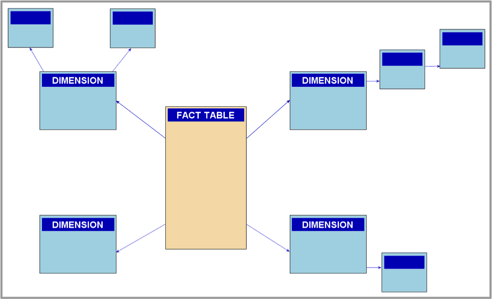
Image 1: snowflake schema example

For such schemas, there are two reasons a bushy tree outperforms any linear “deep” tree:

Parallel execution of independent plan fragments
Reduced intermediary data size

To better understand the impact of join ordering, consider TPC-DS query 17:

select 
    i_item_id,
    i_item_desc,
    s_state,
    count(ss_quantity) as store_sales_quantitycount,
    avg(ss_quantity) as store_sales_quantityave,
    stddev_samp(ss_quantity) as store_sales_quantitystdev,
    stddev_samp(ss_quantity) / avg(ss_quantity) as store_sales_quantitycov,
    count(sr_return_quantity) as store_returns_quantitycount,
    avg(sr_return_quantity) as store_returns_quantityave,
    stddev_samp(sr_return_quantity) as store_returns_quantitystdev,
    stddev_samp(sr_return_quantity) / avg(sr_return_quantity) as store_returns_quantitycov,
    count(cs_quantity) as catalog_sales_quantitycount,
    avg(cs_quantity) as catalog_sales_quantityave,
    stddev_samp(cs_quantity) / avg(cs_quantity) as catalog_sales_quantitystdev,
    stddev_samp(cs_quantity) / avg(cs_quantity) as catalog_sales_quantitycov
from
    store_sales,
    store_returns,
    catalog_sales,
    date_dim d1,
    date_dim d2,
    date_dim d3,
    store,
    item
where
    d1.d_quarter_name = '2000Q1'
        and d1.d_date_sk = ss_sold_date_sk
        and i_item_sk = ss_item_sk
        and s_store_sk = ss_store_sk
        and ss_customer_sk = sr_customer_sk
        and ss_item_sk = sr_item_sk
        and ss_ticket_number = sr_ticket_number
        and sr_returned_date_sk = d2.d_date_sk
        and d2.d_quarter_name in ('2000Q1' , '2000Q2', '2000Q3')
        and sr_customer_sk = cs_bill_customer_sk
        and sr_item_sk = cs_item_sk
        and cs_sold_date_sk = d3.d_date_sk
        and d3.d_quarter_name in ('2000Q1' , '2000Q2', '2000Q3')
group by i_item_id , i_item_desc , s_state
order by i_item_id , i_item_desc , s_state
limit 100;

The query above involves three fact tables: store_sales (82B), store_returns (8B) and catalog_sales (43B). It also involves five dimension tables: date_dim d1 (73K), date_dim d2 (73K), date_dim d3 (73K), store (1.7K) and item (462K).

Graph 5: join graph for TPC-DS Q17

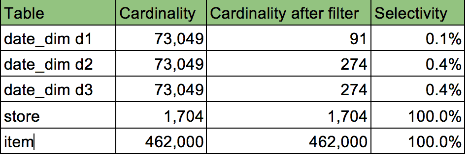
Table 3: dimension table cardinality and selectivity for TPC-DS Q17

From Table 3, it is clear that joining date_dim d1, d2 and d3 should result in a reduction of intermediary rows in the plan, while dimension tables of store and item will provide no reduction in rows, as they have a selectivity of one (1).

Bushy join support: results

CBO ON

Similar to our join ordering optimization scenario, the CBO creates an optimal join graph that reduces intermediary data size. But, in this case, it is able to create a bushy tree instead of a left-deep tree.

The join tree below shows the CBO will join the fact tables with their corresponding date_dim table first, before completing any fact-to-fact joins. The CBO is also able to delay the join of store_sales with the store and item tables. Since the joins with both tables have a selectivity of one (1), the CBO will order the joins such that the selective joins are handled first, followed by the less selective ones.

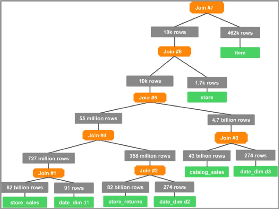
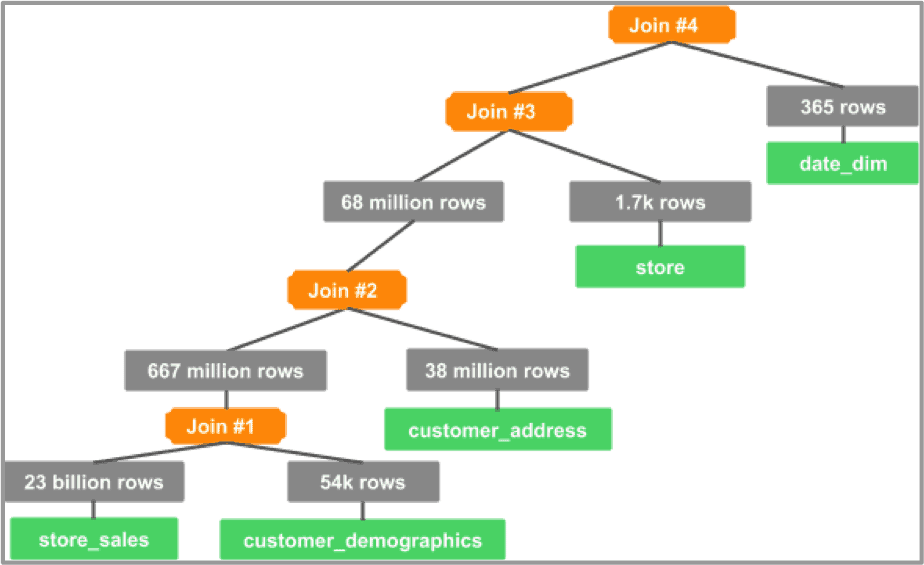
Graph 6: join tree for TPC-DS Q17 with CBO ON

The join tree in Graph 6 shows how the CBO joins each of the fact tables with the most selective corresponding table. This avoids large fact-to-fact joins, which require expensive shuffles. Even after joining with date_dim, the CBO is able to order joins efficiently—as seen in Join #4, which reduces 2.5 billion + 1.2 billion to just 55 million rows.

Store and item tables have a selectivity of one (1), so they are joined last.

There is no point in needing to pass billions of rows through a join operator that will qualify all of the rows.

CBO OFF

Graph 7 shows the join tree with the CBO OFF. Notice how the join tree resembles a left-deep tree. Joins #1 and #2 are large fact-to-fact joins⎯so store_sales, store_returns and catalog_sales are joined together, producing lots of intermediate data. Joins #1 and #2 are executed as shuffle joins when both relations are shuffled on the join keys.

Graph 7: join tree for TPC-DS Q17 with CBO OFF

Bushy join support: interpreting the results

The CBO generates a bushy tree that reduces intermediary data set size. The efficient join order produced by the CBO allows the physical optimizer to reduce the number of rows involved in shuffle joins. This is achieved by creating a map join of the fact table with the corresponding date_dim table, before doing the joins between store_sales, store_returns and catalog_sales.

Table 4 summarizes the impact of the efficient join tree produced by the CBO. It shows a roughly sevenfold speedup in response time, plus a sevenfold reduction in CPU utilization, while the data shuffled over the network is reduced from 1.3 TB to just 78 GB.

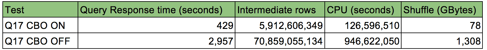
Table 4: elapsed time, intermediate rows and CPU for TPC-DS Q17 with CBO ON vs. OFF

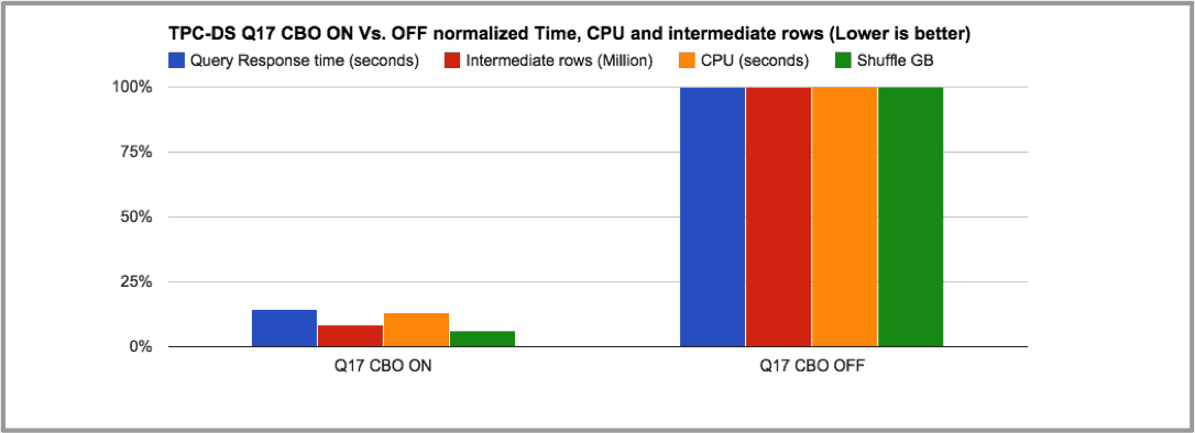
Graph 8: elapsed time and CPU for TPC-DS Q17 with CBO ON vs. OFF

3. Join simplification

Among the new features offered by Hive 0.14 CBO is join predicate simplification. The CBO is able to identify common join predicates from the conjunction and disjunction clause, plus create an implied join predicate, avoiding costly cross-product joins.

An example for this optimization is TPC-DS Q48, which clearly illustrates this issue. Notice the join predicates in bold between customer_demographics x store_sales and store_sales x customer_address.

select 
    sum(ss_quantity)
from
    store_sales,
    store,
    customer_demographics,
    customer_address,
    date_dim
where
        store.s_store_sk = store_sales.ss_store_sk
        and store_sales.ss_sold_date_sk = date_dim.d_date_sk
        and d_year = 1998
        and ((
customer_demographics.cd_demo_sk = store_sales.ss_cdemo_sk
        and cd_marital_status = 'M'
        and cd_education_status = '4 yr Degree'
        and ss_sales_price between 100.00 and 150.00)
        or (
customer_demographics.cd_demo_sk = store_sales.ss_cdemo_sk
        and cd_marital_status = 'M'
        and cd_education_status = '4 yr Degree'
        and ss_sales_price between 50.00 and 100.00)
        or (
customer_demographics.cd_demo_sk = store_sales.ss_cdemo_sk
        and cd_marital_status = 'M'
        and cd_education_status = '4 yr Degree'
        and ss_sales_price between 150.00 and 200.00))
        and ((
store_sales.ss_addr_sk = customer_address.ca_address_sk
        and ca_country = 'United States'
        and ca_state in ('KY' , 'GA', 'NM')
        and ss_net_profit between 0 and 2000)
        or (
store_sales.ss_addr_sk = customer_address.ca_address_sk
        and ca_country = 'United States'
        and ca_state in ('MT' , 'OR', 'IN')
        and ss_net_profit between 150 and 3000)
        or (
store_sales.ss_addr_sk = customer_address.ca_address_sk
        and ca_country = 'United States'
        and ca_state in ('WI' , 'MO', 'WV')
        and ss_net_profit between 50 and 25000))

Join simplification: results and interpretation

CBO ON

The CBO is able to identify that the join predicates (customer_demographics x store_sales and store_sales x customer_address) are duplicated in the three disjunctions. The CBO also simplifies the join tree, avoiding a cross product.
Additionally, the CBO improves performance by simplifying some of the table predicates, while also pushing them down to scan further and reducing the intermediary data size.

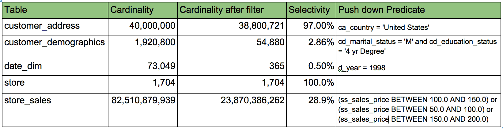
Table 5: table cardinality and selectivity after simplifying and pushing down the column predicates for Q48 with CBO ON

Graph 9: join tree for TPC-DS Q48 with CBO ON

The CBO is able to order joins efficiently while avoiding a cross-product join.

CBO OFF

With the CBO disabled, a cross product generated for store_sales x customer_demographics x customer_address (without any filters) translates to 805 billion x 1.9 million x 40 million = 6.1903E+24 rows. Obviously, this query is not going to finish in a reasonable amount of time.

Conclusion

In this post, we’ve highlighted some of the new query optimizations introduced in Hive 0.14 via Calcite, covering join ordering optimization, bushy join trees, and cross-product elimination. It’s clear that users can expect striking performance gains in query planning by leveraging the Cost-Based Logical Optimizer in Hive 0.14.

Stop Thinking, Just Do!