Article Source
Graph Neural Networks as Neural Diffusion PDEs
At Twitter, our core data assets are huge graphs that describe how users interact with each other through Follows, Tweets, Topics and conversations. These graphs are associated with rich multimedia content and understanding this content and how our users interact with it is one of our core ML challenges. Graph neural networks (GNNs) work by combining the benefits of multilayer perceptrons with message passing operations that allow information to be shared between nodes in a graph. Message passing is a form of diffusion and so GNNs are intimately related to the differential equations that describe diffusion. Thinking of GNNs as discrete partial differential equations (PDEs) leads to a new broad class of architectures. These architectures address, in a principled way, some of the prominent issues of current Graph ML models such as depth, oversmoothing, bottlenecks, and graph rewiring.
*This blog post is based on the paper B. Chamberlain, J. Rowbottom et al., “GRAND: Graph Neural Diffusion” (2021) ICML. James Rowbottom was an intern at Twitter Cortex in 2021. *
In March 1701, the Philosophical Transactions of the Royal Society published an anonymous note in Latin titled “A Scale of the Degrees of Heat” [1]. Though no name was indicated, it was no secret that Sir Isaac Newton was the author. In a series of experiments, Newton observed that
“…the temperature a hot body loses in a given time is proportional to the temperature difference between the object and the environment…”
— a modern statement of a law that today bears his name [2]. Expressed mathematically, Newton’s law of cooling gives rise to the heat diffusion equation, a Partial Differential Equation (PDE) which in the simplest form reads
ẋ= aΔx.
Here, x(u,t) denotes the temperature at time t and point u on some domain. The left-hand side (temporal derivative ẋ) is the “rate of change of temperature”. The right-hand side (spatial second-order derivative or the Laplacian Δx) expresses the local difference between the temperature of a point and its surrounding, where a is the coefficient known as the thermal diffusivity. When a is a scalar constant, this PDE is linear and its solution can be given in closed form as the convolution of the initial temperature distribution with a time-dependent Gaussian kernel [3],
| x(u,t) = x(u,0)﹡exp(− | u | ²/4t). |
More generally, the thermal diffusivity varies in time and space, leading to a PDE of the form
ẋ(u,t) = div(a(u,t)∇x(u,t))
encoding the more general Fourier’s heat transfer law [4].

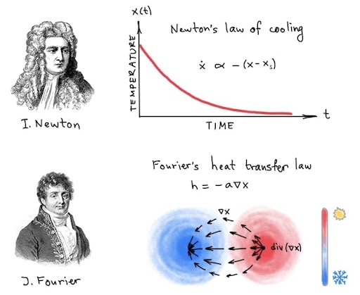
According to Newton’s law of cooling (top), the rate of change of the temperature of a body (ẋ) is proportional to the difference between its own temperature and that of the surrounding. The solution of the resulting differential equation has the form of exponential decay. Fourier’s heat transfer law (bottom) provides a more granular local model:
- The temperature is a scalar field x
- The scalar field’s negative gradient is a vector field −∇x, representing the flow of heat from hotter regions (red) to colder ones (blue)
- The divergence div(−∇x) is the net flow of the vector field −∇x through an infinitesimal region around a point
| Diffusion PDEs arise in many physical processes involving the transfer of “stuff” (whether energy or matter), or more abstractly, information. In image processing, one can exploit this interpretation of diffusion as linear low-pass filtering for image denoising. However, such a filter, when removing noise, also undesirably blurs transitions between regions of different color or brightness (“edges”). An influential insight of Pietro Perona and Jitendra Malik [5] was to consider an adaptive diffusivity coefficient inversely dependent on the norm of the image gradient | ∇x | . This way, diffusion is strong in “flat” regions (where | ∇x | ≈0) and weak in the presence of brightness discontinuities (where | ∇x | is large). The result was a nonlinear filter capable of removing noise from the image while preserving edges. |

Left: original image of Sir Isaac Newton, middle: Gaussian filter, right: nonlinear adaptive diffusion.
Perona-Malik diffusion and similar schemes created an entire field of PDE-based techniques that also drew inspiration and methods from geometry, calculus of variations, and numerical analysis [6,7]. Variational and PDE-based methods dominated the stage of image processing and computer vision for nearly twenty years, ceding to deep learning in the second decade of the 2000s [8].
Diffusion equations on graphs
In our recent work [9], we relied on the same philosophy to take a fresh look at graph neural networks. GNNs operate by exchanging information between adjacent nodes in the form of message passing, a process that is conceptually equivalent to diffusion. In this case, the base space is the graph and the diffusion happens along edges, where the analogy of the spatial derivatives is the differences between adjacent node features.
Formally, the generalization of diffusion processes to graphs is almost straightforward. The equation looks identical:
Ẋ(t) =div(A(X(t))∇X(t))
Where:
- X(t) is now an n×d matrix of node features at time t
- The gradient is an operator assigning to each edge u~v the difference of the respective node feature vectors, (∇X)ᵤᵥ=xᵥ−xᵤ
- The divergence at node v sums the features of edges emanating from v, ∑ᵥ wᵤᵥ xᵤᵥ [10]
The diffusivity is represented by a matrix-valued function of the form A(X)=diag(a(xᵤ, xᵥ)), where, as before, a is a function determining the strength of diffusion along edge u~v based on the similarity of the respective features xᵤ and xᵥ [11]. The graph diffusion equation can be written conveniently as a matrix differential equation of the form:
Ẋ(t) =(A(X(t))−I)X(t).
In most cases [12], this differential equation has no closed-form solution and has to be solved numerically. There are many numerical techniques for solving nonlinear diffusion equations, differing primarily in the choice of spatial and temporal discretization.
The simplest discretization replaces the temporal derivative Ẋ with the forward time difference:
[X(k+1)−X(k)]/𝜏=[A(X(k))−I]X(k)
where k denotes the discrete time index (iteration number) and 𝜏 is the step size such that t=k𝜏. Rewriting the above formula as:
X(k+1)=[(1−𝜏)I+𝜏A(X(k))]X(k)=Q(k)X(k)
we get the formula of an explicit or forward Euler scheme, where the next iteration X(k+1) is computed from the previous one X(k) by applying a linear operator Q(k) [13], starting from some X(0). This scheme is numerically stable (in the sense that a small perturbation in the input X(0) results in a small perturbation to the output X(k)) only when the time step is sufficiently small, 𝜏<1.
Using backward time difference to discretize the temporal derivative leads to the (semi-)implicit scheme:
[(1+𝜏)I−𝜏A(X(k))]X(k+1)=B(k)X(k+1)=X(k)
The scheme is called “implicit” because deducing the next iterate from the previous one requires solving a linear system amounting to the inversion of B. In most cases, this is carried out approximately, by a few iterations of a linear solver. This scheme is unconditionally stable, meaning that we can use any 𝜏>0 without worrying that the iterations will “blow up”.
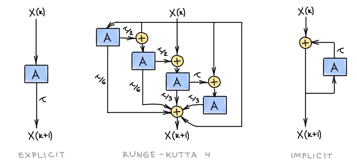
These conceptually simple discretization techniques do not necessarily work well in practice. In the PDE literature, it is common to use multi-step schemes such as Runge-Kutta [14] where the subsequent iterate is computed as a linear combination of a few previous ones. Both the explicit and implicit cases can be made multi-step. Furthermore, the step size can be made adaptive, depending on the approximation error [15].
 Left-to-right: single step explicit Euler, multi-step fourth-order Runge-Kutta, single step implicit. A denotes the diffusion operator;𝜏 is the time step size.
Diffusion equations with a parametric diffusivity function optimized for a given task define a broad family of graph neural network-like architectures we call Graph Neural Diffusion (or, somewhat immodestly, GRAND for short). The output is the solution X(T) of the diffusion equation at some end time T. Many popular GNN architectures can be formalized as instances of GRAND , for example, parametric discretized graph diffusion equations. Specifically, the explicit scheme mentioned above has the form of a Graph Attention Network [16], where our diffusivity plays the role of attention.
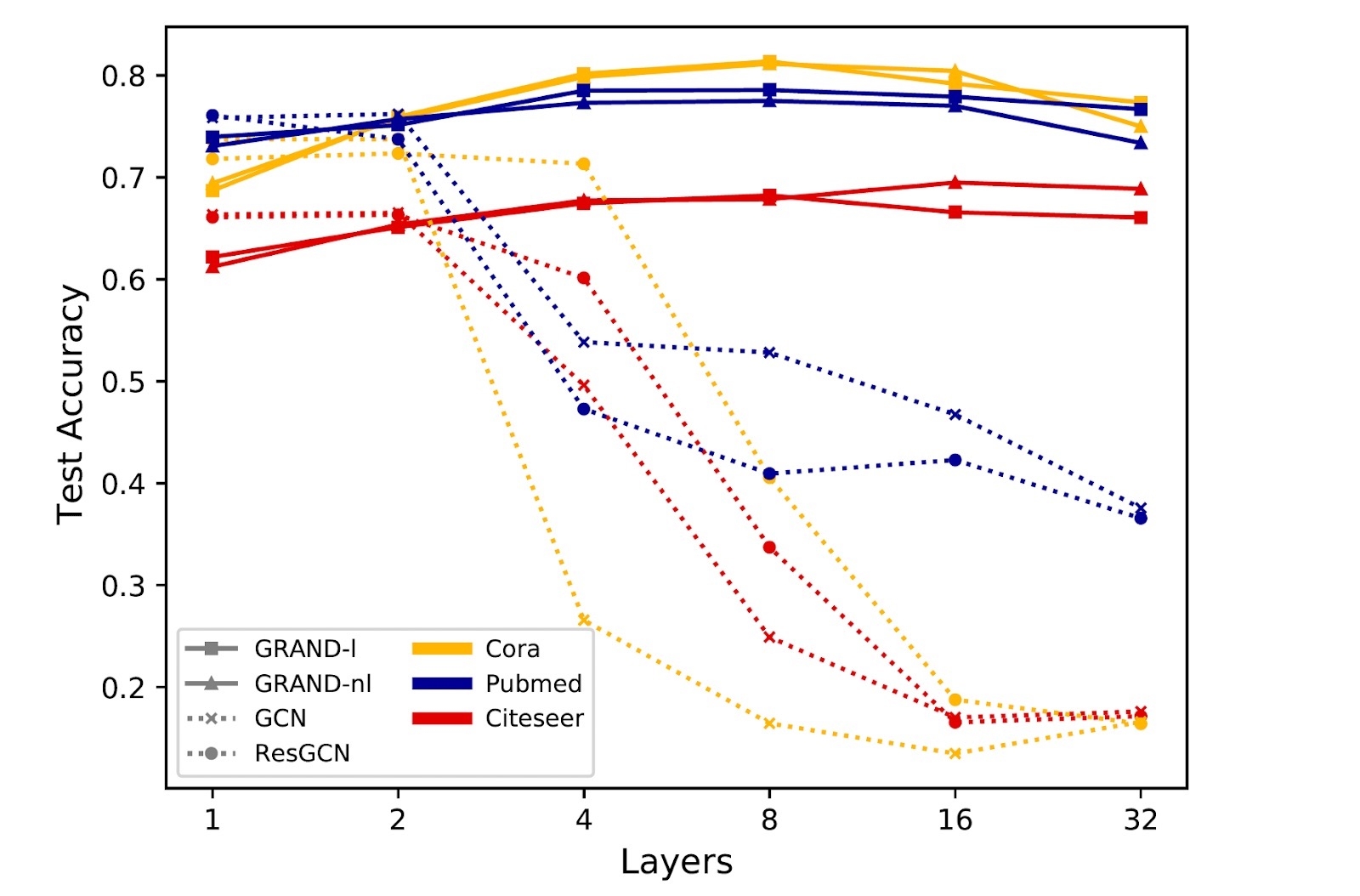
The vast majority of GNNs use the explicit single-step Euler scheme. In this scheme, the discrete time index k corresponds to a convolutional or attentional layer of the graph neural network. Running the diffusion for multiple iterations amounts to applying a GNN layer multiple times. In our formalism, the diffusion time parameter t acts as a continuous analogy of the layers [17] — an interpretation allowing us to exploit more efficient and stable numerical schemes that use adaptive steps in time. In particular, GRAND allows addressing the widely recognised problem of degradation of performance in deep GNNs.
 In Graph Neural Diffusion, explicit GNN layers are replaced with the continuous analog of diffusion time. This scheme allows training deep networks without experiencing performance degradation.
Implicit schemes allow using larger time steps and thus less iterations (“layers”) at the expense of the computational complexity of the iteration, which requires the inversion of the diffusion operator. The diffusion operator (the matrix A in our notation) has the same structure of the adjacency matrix of the graph (1-hop filter), while its inverse is usually a dense matrix that can be interpreted as a multi-hop filter.
Since the efficiency of matrix inversion crucially depends on the structure of the matrix, in some situations it might be advantageous to decouple the graph used for diffusion from the input graph. Such techniques, collectively known as graph rewiring, have become a popular approach to deal with scalability or information bottlenecks in GNNs. The diffusion framework offers a principled view on graph rewiring by considering the graph as a spatial discretization of some continuous object (for example, a manifold) [18]. This principled view on graph rewiring is also because some discretizations are more advantageous numerically.
 Discretizations of the 2D Laplacian operator. Any convex combination of discretizations is also a valid one. Choosing a discretization is a Euclidean analogy of “graph rewiring”.
Conclusion
Graph Neural Diffusion provides a principled mathematical framework for studying many popular architectures for deep learning on graphs as well as a blueprint for developing new ones. This mindset sheds new light on some of the common issues of GNNs such as feature over-smoothing and the difficulty of designing deep neural networks and heuristic techniques such as graph rewiring. More broadly, we believe that exploring the connections between graph ML, differential equations, and geometry and leveraging the vast literature on these topics will lead to new interesting results in the field.
References
[1] Anonymous, Scala graduum Caloris. Calorum Descriptiones et signa (1701) Philosophical Transactions 22 (270): 824–829.
[2] E. F. Adiutori, Origins of the heat transfer coefficient (1990) Mechanical Engineering argues that Newton should not be credited with the discovery of the law bearing his name, and the honour should be given to Joseph Black and Joseph Fourier instead.
[3] This is easy to see by expanding x in a Fourier series and plugging it into both sides of the equation. Solving heat equations was one of the motivations for the development of this apparatus by J. Fourier, Théorie analytique de la chaleur (1824), which today bears his name.
[4] According to Fourier’s law, the thermal gradient ∇x creates a heat flux h=−a∇x satisfying the continuity equation ẋ=−div(h). This encodes the assumption that the only change in the temperature is due to the heat flux (as measured by the divergence operator). That is, heat is not created or destroyed.
[5] P. Perona and J. Malik, “Scale-space and edge detection using anisotropic diffusion” (1990), PAMI 12(7):629–639.
[6] J. Weickert, Anisotropic Diffusion in Image Processing (1998) Teubner.
[7] R. Kimmel, Numerical Geometry of Images (2004) Springer.
[8] PDE-based and variational methods are linked because PDEs can be derived as the optimality conditions (known as Euler-Lagrange equations) of some functional measuring the “quality” of the resulting image. The homogeneous diffusion equation, for example, is a minimising flow (roughly, a continuous analogy of gradient descent in variational problems) of the Dirichlet energy. The paradigm of designing a functional, deriving a PDE minimising it, and running it on an image is conceptually very appealing. However, most “handcrafted” functionals are often idealized and show inferior performance compared to deep learning, which explains the demise of PDE-based methods in the past decade.
[9] B. Chamberlain, J. Rowbottom et al., GRAND: Graph Neural Diffusion (2021) ICML. Different flavors of graph diffusion equations have been used before in many applications. In the GNN literature, diffusion equations were mentioned in F. Scarselli et al., The graph neural network model (2009) IEEE Trans. Neural Networks 27(8):61–80 as well as more recently J. Zhuang, Ordinary differential equations on graph networks (2019) arXiv:1911.07532, F. Gu et al., Implicit graph neural networks (2020) NeurIPS, and L.-P. Xhonneux et al., Continuous graph neural networks (2020) ICML.
[10] We use a standard notation: the graph G has n nodes and m edges, W is the n×n adjacency matrix with wᵤᵥ=1 if u~v and zero otherwise. Given d-dimensional node features arranged into an n×d matrix X, the gradient ∇X can be represented as a matrix of size m×d. Similarly, given edge features matrix Y of size m×d, the divergence div(Y) is an n×d matrix. The two operators are adjoint with regards to the appropriate inner products, ⟨∇X,Y⟩=⟨X,div(Y)⟩. We slightly abuse the notation denoting by xᵤ the node features (analogous to scalar fields in the continuous case) and by xᵤᵥ the edge features (analogous to vector fields). The distinction is clear from the context.
[11] We assume A is normalised, ∑ᵥ aᵤᵥ=1.
[12] For a constant A, the solution of the diffusion equation can be written in closed form as X(t)=exp(t(A−I))X(0)=exp(tΔ)X(0). The exponential of the graph Laplacian Δ is known as the heat kernel and can be interpreted as a generalized (spectral) convolution with a low-pass filter.
[13] Note that Q is dependent on X (and thus changes every iteration) but its application to X is linear and takes the form of a matrix product. This has an exact analogy to the “attentional” flavor of GNNs.
[14] Named after C. Runge, Über die numerische auflösung von differentialgleichungen (1895) Mathematische Annalen 46(2):167–178 and W. Kutta, Beitrag zur naherungsweisen integration totaler differentialgleichungen (1901) Z. Math. Phys. 46:435–453, the Runge-Kutta method is actually not a single scheme but a class of numerical schemes. Specifically, in our paper we used the popular Dormand-Prince scheme.
[15] Typically the approximation error is computed as the difference between two subsequent approximation orders.
[16] P. Veličković et al., Graph Attention Networks (2018) ICLR. More specifically, we assume no nonlinearity between layers and shared attention parameters across layers (corresponding to time-independent diffusivity). The latter is a big advantage: in our experiments, we obtained results superior in most cases to those of GAT while using up to 20× less parameters.
[17] “Neural ODEs”, or the interpretation of residual neural networks as Euler discretization of an ordinary differential equation, was proposed by several groups, including E. Haber and L. Ruthotto, Stable architectures for deep neural networks (2017) Inverse Problems 34 (1), Y. Lu et al., Beyond finite layer neural networks: bridging deep architectures and numerical differential equations (2018) ICML, and perhaps the most famous of them all, R. Chen et al., Neural Ordinary Differential Equations (2019) NeurIPS. Our approach can be considered as “Neural PDEs”.
[18] This is certainly the case for scale-free graphs such as social networks that can be realized in spaces with hyperbolic geometry. Geometric interpretation of graphs as continuous spaces is the subject of the field of network geometry, see e.g. M. Boguñá et al., Network geometry (2021) Nature Reviews Physics 3:114–135.
We are grateful to James Rowbottom, Nils Hammerla, Ramia Davis, and Peyman Milanfar for their comments.